Model Simulation - Part II
Model Simulation (II)
1. Simple Model Comparison - Page 1/2
As explained in Unit 7, by repeated simulations it is possible to obtain deepen insight into the model under consideration. This can be useful for model comparison.
Example 8.1. Basic vs Time-dependent IFM, whitout rescue effect.
We use simulations to compare the basic and the time-dependent IFM. This Example is analogous to Example 7.3: as far as the time-dependent model is concerned, simulations are obtained by applying the function “sim1TD” of Example 7.2. Let be simTtd the analogous of simT in Example 7.3.
simTtd[1:13,]/ns
[,1] [,2] [,3] [,4] [,5] [,6] [,7] [,8] [,9] [,10] [,11]
[1,] 1 0.2493 0.7633 0.4113 0.6500 0.4922 0.5962 0.5236 0.5834 0.5349 0.5689
[2,] 0 0.9999 0.3364 0.7789 0.4869 0.6775 0.5440 0.6308 0.5783 0.6144 0.5912
[3,] 1 0.2427 0.8169 0.3851 0.7068 0.4677 0.6517 0.5073 0.6098 0.5363 0.5877
[4,] 0 0.9998 0.2916 0.7908 0.4311 0.6900 0.5145 0.6389 0.5466 0.6130 0.5672
[5,] 0 0.9985 0.3026 0.7879 0.4476 0.6778 0.5233 0.6351 0.5559 0.6128 0.5652
[6,] 0 1.0000 0.3473 0.7699 0.4846 0.6752 0.5553 0.6334 0.5794 0.6242 0.5878
[7,] 0 0.7643 0.4276 0.5817 0.5043 0.5454 0.5331 0.5350 0.5400 0.5308 0.5317
[8,] 1 0.2883 0.7963 0.4304 0.6952 0.5057 0.6396 0.5507 0.6096 0.5689 0.5973
[9,] 1 0.3198 0.7826 0.4757 0.6752 0.5432 0.6291 0.5852 0.6056 0.5892 0.6006
[10,] 1 0.3503 0.7710 0.5020 0.6727 0.5676 0.6352 0.5917 0.6223 0.5957 0.6146
[11,] 1 0.3328 0.7752 0.4689 0.6876 0.5379 0.6390 0.5737 0.6146 0.5820 0.6100
[12,] 1 0.2864 0.7792 0.4367 0.6695 0.5138 0.6187 0.5565 0.5953 0.5709 0.5787
[13,] 0 0.9995 0.3343 0.7750 0.4864 0.6736 0.5514 0.6262 0.5831 0.6127 0.5929
# This output excerpt looks quite similar to the analogous in
# Example 7.3
plot((simTtd[,5]-simT[,5])/ns,type="o",lwd=2,xlab="t",ylab="t=5", main="T.D. IFM - BASIC IFM")
abline(h=0, col="red")
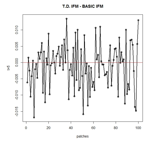
# in fact, the greater difference is lower than 0.02
max(abs((simTtd[,5]-simT[,5])/ns))
[1] 0.0169
In Example 8.1 the basic and the time-dependent IFM have been compared by looking at the approximated probabilities P(Xt(i) = 1) for t = 2,…,11 and i = 1,…,100. Now we consider something similar to Figure 7.2, as mentioned at the end of Unit 7. Rescue effect is not considered here.
We focus on the number of occupied sites a different times t. For each model, we generate many simulations like those in Figure 7.2 (black and blue lines) and at each time t we compare the distributions of the number of occupied sites coming from the two models.
Example 8.2. Basic vs Time-dependent IFM, whitout rescue effect.
Instructions will be explicitly given for the basic model, as for the time-dependent model the procedure is exactly the same except for applying sim1TD (see Example 7.2) instead of sim1.
# For the basic IFM:
pm<-(p+p1)/2
S<-rowSums(edis[,pm>0])
C<-S^2/(S^2+yhat^2)
ns=10000 # number of simulations
nt=10 # length of the simulated period
# each row of nsites1 will contain “a black line” (see Figure of
# Example 7.2)
nsites1<-matrix(0,nrow=ns, ncol=nt+1)
for(k in 1:ns) {
sim<-matrix(0,nrow=length(p1),ncol=nt+1)
sim[,1]<-p1
for(t in 1:nt) sim[ ,t+1]<-sim1(sim[ ,t])
nsites1[k,]<-colSums(sim)
}
nsites1[1:5,]
[,1] [,2] [,3] [,4] [,5] [,6] [,7] [,8] [,9] [,10] [,11]
[1,] 61 46 64 49 54 57 53 60 47 66 48
[2,] 61 47 63 47 58 55 58 51 60 55 55
[3,] 61 51 59 58 50 59 51 53 59 52 53
[4,] 61 48 62 45 61 56 54 63 49 54 55
[5,] 61 47 62 53 53 59 57 49 50 60 55
median1<-c()
for (k in 1nt+1)) median1<-c(median1,median(nsites1[,k]))
# a box-plot for each column of nsites1 is drawn, and the medians
# connected by a red line
boxplot(nsites1 , xlab="t",ylab="n. occupied sites", main="BASIC IFM")
points(median1,col="red",type="o",lwd=3)
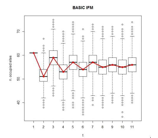
A matrix “nsites2” is obtained by applying “sim1TD”, and the median number of occupied sites per year collected in the vector “median2”. The next picture compares the year-by-year distributions under the two models.
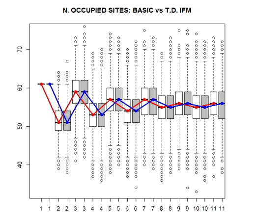
The white box-plots correspond to the basic IFM, as in the previous picture, while the gray boxplots to the time-dependent model (and the blue line connects their medians). This picture clearly shows that when the variability of the simulations is taken into account, the number of occupied sites per year seems behave in the same manner under the two models.
This picture has been obtained by the following instructions:
boxplot(nsites1, xlab="",ylab="", main="N. OCCUPIED SITES: BASIC vs T.D. IFM", at=2*c(1nt+1)))
boxplot(nsites2, , col="gray", at=1+2*c(1nt+1)), add=T)
points(2*c(1nt+1)), median1, col="red", type="o", lwd=3)
points(1+2*c(1nt+1)), median2, col="blue", type="o", lwd=3)
# where the option at determines where to draw each boxplot, while the
# option add=T says that the new boxplots should be drawn together
# with the current ones.
Both the colored lines in the pictures of Example 8.2 suggest that as t increases, the median of the number of occupied sites asymptotically converges to some value, and the corresponding boxplots tend to align themselves. This was expected for the basic IFM, due to the stationary property of the process (see Unit 3 and Eq. (4.1)).