To gain further insight into the role of the IFM parameters we will use simulations to analyze the effect of moving from the “true” parameters (those used to create our reference metapopulation of Example 4.1, and also used in all the previous examples) to different parameter values. This will help us to figure out the role of parameters, and especially the effects of get wrong parameters estimates. Formal parameter estimation will be considered in Units 10 and 11.
Remind that under the basic IFM, the presence/absence of the species at patch i evolves as a Markov Chain with extinction probability
|
|
| Ei = (A0/Ai )x |
if Ai > A0 |
|
| Ei = 1 |
if Ai ≤ A0 |
|
and colonization probability
|
|
| \(C_i(t)=\frac{S_i(t)^2}{S_i(t)^2 + y^2}\) |
|
where
|
|
| \(S_i=\sum_{k \neq i} \bar\delta_i exp(\alpha d_{ik})A_k\) |
|
In all the Units we used as a reference metapopulation presence/absence data obtained by simulations from an IFM at equilibrium with parameters A0 = 0.0004, x = 0.05 and y = 0.005. We will consider variations of one parameter at a time.
Example 9.1. Extinction probabilities, I.
We show by simulations the effect of varying parameter A0. We will refer, as usual, to the metapopulation data of Examples 4.1. In all the previous examples A0 = 0.0004 (Km2). This value is lower than the minimum patch area
> min(A)
and therefore, in all the previous examples Ei < 1 for all i. Let
A0a<-0.0004
and consider a greater value, like
(A0b<-quantile(A,0.25))
that is a value such that the 25% of the smallest patches has patch area lower than A0b. The extinction probabilities increases (compare to Figure 4.1):
summary(Ea)
summary(Eb)
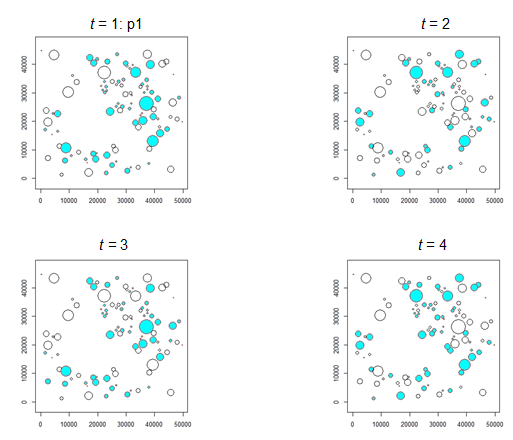
and the smaller patches have Ei = 1. This affects metapopulation dynamics, as shown in the following picture, obtained with analogous instructions than in Example 8.2 (computation of S and C based on pm) 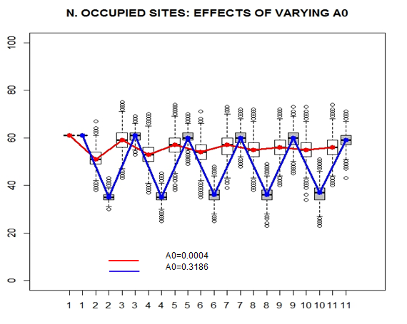
It can be seen that the higher value of A0 yields a more oscillating dynamic (blue line). This oscillation reduces over a very long term period (see Exercise 9.3). Let’s look to some consecutive metapopulation snapshots to figure out the spatial evolution when A0 = 0.3186.
nt=3;
sim<-matrix(0,nrow=length(p),ncol=nt+1)
sim[,1]<-p1
for(t in 1:nt) sim[ ,t+1]<-sim1(sim[ ,t]) # sim1 is based on A0b
sim[1:5,]
op <- par(mfrow = c(2,2), pty="s")
for(k in 1:4){<br /> plot(x.crd,y.crd,asp=1,xlab="",ylab="",cex=sqrt(A*3),pch=21,<br /> col=sim[,k]+1,bg=5*sim[,k])<br /> }
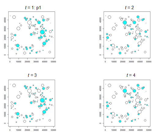
The first picture in Example 9.1 shows a noteworthy feature of the model with A0=0.3186. The blue line oscillates between a minimum value of less than 40 occupied patches to a maximum value of even more than 60 occupied patches. Let’s consider the mean in place of the median, for the sake of simplicity.
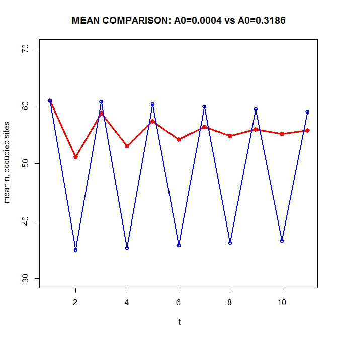
Figure 9.10 – Yearly mean number of occupied sites: A0=0.0004 (red line) versus A0=0.3186 (blue line). Number of simulations: 10,000.
Figure 9.1 shows that, at least over a short period, the expected number of occupied patches under the model with higher extinction probabilities can be higher than under the original model.
This is certainly due to colonization: the two models share the same colonization probabilities that are very high:
The fact that at a given point in time many empty patches are available for colonization yields a high number of occupied patches at the following time
Example 9.2. Extinction probabilities, I.
We show by simulations the effect of varying parameter x.
The extinction probabilities then increases (compare with Figure 4.1):
summary(E)
summary(Ep)
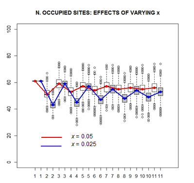
By proceeding as in Example 9.1, we obtain similar results, with a smaller oscillation of the yearly median number of occupied patches.
By the following two examples we move onto colonization probabilities.
9.3. Colonization probabilities, I.
We show by simulations the effect of varying parameter \(\alpha\).
In the previous examples \(\alpha\) = 1. Let now \(\alpha\)' = 2, that is
alpha<-1 # yielding col. prob. C
alphap<-2 # yielding col. prob. Cp
Mortality rate is increased and therefore, colonization probabilities are decreased (as connectivity decrease).
summary(C)
summary(Cp)
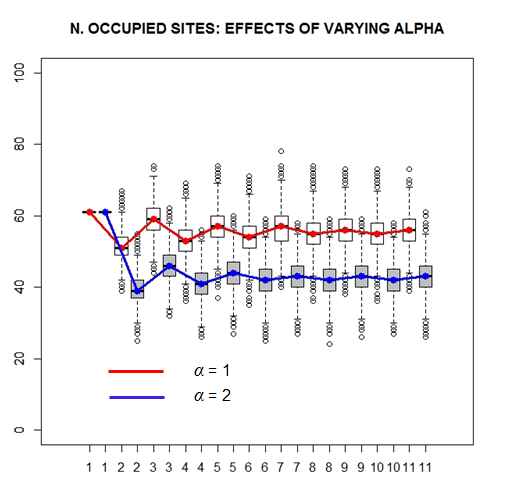
This picture shows that increasing the mortality rate strongly affects the dynamics by significantly reducing the number of occupied patches at each time, in contrast with Examples 9.1 and 9.2 where extinction probabilities are enhanced.
9.4. Colonization probabilities, II.
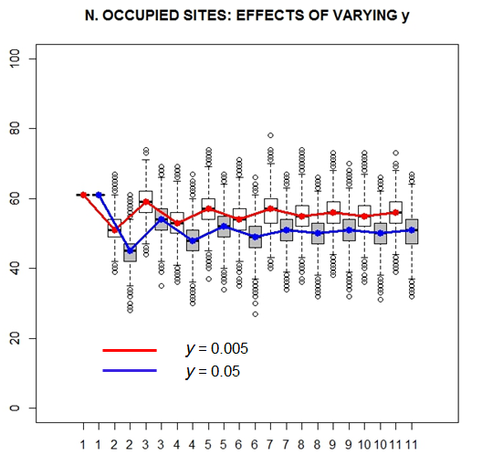
We show by simulations the effect of varying parameter y.
In the previous examples y = 0.005. Let now y = 0.05, that is
yhat<-0.005 # yielding col. prob. C
yphat<-0.05 # yielding col. prob. Cp
Colonization probabilities are directly decreased, while connectivity do not change.
Cp<-S^2/(S^2+yphat^2)
summary(C)
summary(Cp)
The result is, however, similar.
Example 8.2 shows that for the usual choice of the model parameters: x = 0.05, y = 0.005, \(\alpha\)= 1 and A0 = 0.004, the yearly number of occupied patches is very similar under the basic and the time-dependent IFM. For this reason, we will not go through an analogous sequence of examples for the time-dependent model. We limit ourselves to compare, in Figure 9.2, the basic and the time-dependent model when a higher value for parameter A0 is considered. The picture shows that increasing the critical patch area has a lower effect on the time-dependent model, in the sense that the oscillation of the number of occupied sites is slightly reduced, due to effect of time-varying connectivity (and therefore, of colonization probabilities).
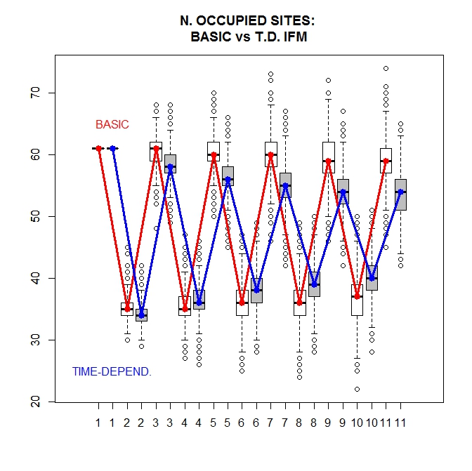
Figure 9.2 – Considering a higher critical patch area as in Example 9.1 has a lower effect on the time-dependent model rather than on basic model, in the sense that the oscillation of the number of occupied sites is slightly reduced.