Data Management and Biodiversity partitioning using the R package entropart - Gestione dati e partizione della biodiversità con il package entropart di R
Data Management and Biodiversity partitioning using the R package entropart - Gestione dati e partizione della biodiversità con il package entropart di R
Diversity partitioning
Tsallis γ entropies and diversity are easily partitioned into α and β components using the entropart package functions:- GammaEntropy() and GammaDiversity()
- AlphaEntropy() and AlphaDiversity()
- BetaEntropy() and BetaDiversity()
- DivPart is a function combining all the above functions
Notice that all α and β functions return lists with vector elements:
> AlphaEntropy(Meta.jv,q=1) ##a list with several information
$MetaCommunity [1] "Meta.jv"
$Type
[1] "alpha"
$Order
[1] 1
$Correction
[1] "Best"
$Normalized
[1] TRUE
$Weights
| Allaine | Audeux | Clauge | Cuisance | Cusancin | Dessoubre | Doubs | Doulonnes | Drugeon | Furieuse | Lison | Loue |
| 0.03815114 | 0.02714600 | 0.09097579 | 0.05282465 | 0.02714600 | 0.03888481 | 0.22157007 | 0.02567865 | 0.07043287 | 0.04842260 | 0.05869406 | 0.30007337 |
| Allaine | Audeux | Clauge | Cuisance | Cusancin | Dessoubre | Doubs | Doulonnes | Drugeon | Furieuse | Lison | Loue |
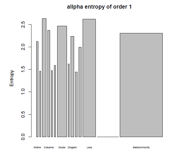
| 2.122794 | 1.461630 | 2.632026 | 2.371961 | 1.474779 | 1.587543 | 2.465101 | 1.620635 | 2.235162 | 1.443209 | 1.994400 | 2.616050 |
$Total [1] 2.304366 attr(,"class") [1] "MCentropy"
> summary(AlphaEntropy(Meta.jv,q=1))
alpha Entropy of order 1 of MetaCommunity Meta.jv with correction: Best Entropy of communities:
| Allaine | Audeux | Clauge | Cuisance | Cusancin | Dessoubre | Doubs | Doulonnes | Drugeon | Furieuse | Lison | Loue |
| 2.122794 | 1.461630 | 2.632026 | 2.371961 | 1.474779 | 1.587543 | 2.465101 | 1.620635 | 2.235162 | 1.443209 | 1.994400 | 2.616050 |
Average entropy of the communities: [1] 2.304366
Notice that
> GammaEntropy(Meta.jv,q=1,Correction="ChaoShen")
[1] 2.55195
returns only one value and the same value obtained running the Shannon() function. Some difference is observed if the option Correction="Best" is specified in the GammaEntropy function.> summary(BetaEntropy(Meta.jv,q=1))
beta Entropy of order 1 of MetaCommunity Meta.jv with correction: Best Entropy of communities:
| Allaine | Audeux | Clauge | Cuisance | Cusancin | Dessoubre | Doubs | Doulonnes | Drugeon | Furieuse | Lison | Loue |
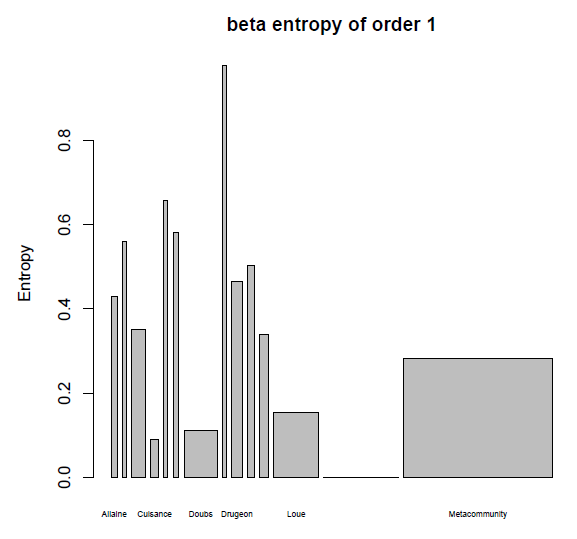
| 0.42878299 | 0.56022760 | 0.35113958 | 0.08872304 | 0.65779757 | 0.58187935 | 0.11023280 | 0.97903461 | 0.46637253 | 0.50276549 | 0.33853664 | 0.15493055 |
Average entropy of the communities: [1] 0.2817997
To build plots it is more convenient to assign functions outputs to objects:
> alpha.jv=AlphaEntropy(Meta.jv,q=1)
> beta.jv=BetaEntropy(Meta.jv,q=1)
> plot(alpha.jv,cex.names=0.5,main="allpha entropy of order 1")
> plot(beta.jv,cex.names=0.5,main="beta entropy of order 1")
Notice the effects of Bias correction on the diversity measure corresponding to the Shannon entropy:
> GammaDiversity(Meta.jv,q=1,Correction="Best")
[1] 12.87772
> GammaDiversity(Meta.jv,q=1,Correction="ChaoShen")
[1] 12.83211
Diversity partitioning is implement in the function DivPart with no bias correction chosen by default. The option Bias=F has to be set in the function to apply a correction and defaults to the \Best" correction. Other bias corrections can be selected by the Correction option. The syntax is:
> DivPart(q=1,MC=Meta.jv,Bias=TRUE)
$MetaCommunity [1] "Meta.jv" $Order [1] 1 $Biased [1] TRUE $Correction [1] "Best" $Normalized [1] TRUE $TotalAlphaDiversity 12 [1] 9.471408 $TotalBetaDiversity [1] 1.354824 $GammaDiversity [1] 12.83209 $CommunityAlphaDiversities
| Allaine | Audeux | Clauge | Cuisance | Cusancin | Dessoubre | Doubs | Doulonnes | Drugeon | Furieuse | Lison | Loue |
| 7.240207 | 3.886486 | 12.740403 | 9.499748 | 3.861617 | 4.624712 | 11.340470 | 4.711500 | 8.804402 | 3.773609 | 6.725789 | 13.545080 |
$TotalAlphaEntropy [1] 2.248278 $TotalBetaEntropy [1] 0.3036712 $GammaEntropy [1] 2.551949 $CommunityAlphaEntropies
| Allaine | Audeux | Clauge | Cuisance | Cusancin | Dessoubre | Doubs | Doulonnes | Drugeon | Furieuse | Lison | Loue |
| 1.979650 | 1.357505 | 2.544778 | 2.251265 | 1.351086 | 1.531414 | 2.428378 | 1.550006 | 2.175252 | 1.328032 | 1.905949 | 2.606023 |
$CommunityBetaEntropies
| Allaine | Audeux | Clauge | Cuisance | Cusancin | Dessoubre | Doubs | Doulonnes | Drugeon | Furieuse | Lison | Loue |
| 0.4181963 | 0.5601920 | 0.3851946 | 0.1574901 | 0.7774108 | 0.6124040 | 0.1181721 | 1.0542939 | 0.4618816 | 0.6169071 | 0.3666474 | 0.1567946 |
attr(,"class") [1] "DivPart"
> DivPart(q=1,MC=Meta.jv,Bias=FALSE)
$MetaCommunity [1] "Meta.jv" $Order [1] 1 $Biased [1] FALSE $Correction [1] "Best" $Normalized [1] TRUE $TotalAlphaDiversity [1] 10.01783 $TotalBetaDiversity [1] 1.28548 $GammaDiversity [1] 12.87772 $CommunityAlphaDiversities
| Allaine | Audeux | Clauge | Cuisance | Cusancin | Dessoubre | Doubs | Doulonnes | Drugeon | Furieuse | Lison | Loue |
| 8.354445 | 4.312985 | 13.901902 | 10.718386 | 4.370071 | 4.891716 | 11.764667 | 5.056298 | 9.347999 | 4.234261 | 7.347792 | 13.681575 |
$TotalAlphaEntropy [1] 2.304366 $TotalBetaEntropy [1] 0.2511324 $GammaEntropy [1] 2.555498 $CommunityAlphaEntropies
| Allaine | Audeux | Clauge | Cuisance | Cusancin | Dessoubre | Doubs | Doulonnes | Drugeon | Furieuse | Lison | Loue |
| 2.122794 | 1.461630 | 2.632026 | 2.371961 | 1.474779 | 1.587543 | 2.465101 | 1.620635 | 2.235162 | 1.443209 | 1.994400 | 2.616050 |
$CommunityBetaEntropies [1] NA attr(,"class") [1] "DivPart"
Observe that when any correction is applied, no community beta entropies are returned. The returned object is of class \DivPart" and both summary and plot, have methods for it:
> divP.jv=DivPart(q=1,MC=Meta.jv,Bias=FALSE) > summary(divP.jv)
Diversity partitioning of order 1 of MetaCommunity Meta.jv with correction: Best Alpha diversity of communities:
| Allaine | Audeux | Clauge | Cuisance | Cusancin | Dessoubre | Doubs | Doulonnes | Drugeon | Furieuse | Lison | Loue |
| 8.354445 | 4.312985 | 13.901902 | 10.718386 | 4.370071 | 4.891716 | 11.764667 | 5.056298 | 9.347999 | 4.234261 | 7.347792 | 13.681575 |
Total alpha diversity of the communities: [1] 10.01783 Beta diversity of the communities: [1] 1.28548 Gamma diversity of the metacommunity: [1] 12.87772
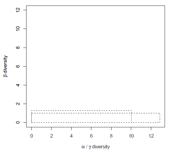
In the plot of the diversity partition of the meta-community Meta.jv, the long rectangle of height 1 represents γ diversity, equal to about 12 effective species. The narrower and higher rectangle has the same area: its horizontal size is α diversity (about 10 effective species) and its height is β diversity (1.354 effective communities).
> plot(divP.jv)
For the macroloire example we have:
> plot(DivPart(q=1,MC=Meta.dat2))
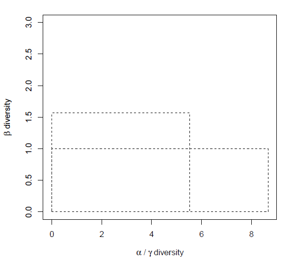
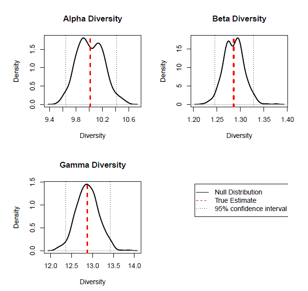
Here the γ-diversity is 8.66 (about 9 effective species), the total α-diversity is 5.52 (about 6 effective species) and the β-diversity is 1.57 (effective communities). If we assume that community species counts are a realization of a multinomial probability distribution, they can be resampled from such distribution to obtain simulated entropies. The function DivEst estimates α, β and γ diversities and their confidence intervals obtained by simulation. It requires the order of the diversity (the corresponding Tsallis entropy), the meta-community, the number of simulations [2], the choice of a bias correction (TRUE or FALSE) and the name of the correction.
> divE.jv=DivEst(q=1,MC=Meta.jv,Simulations=500,Biased=FALSE,Correction="Best")
==============================================================================
> plot(divE.jv)
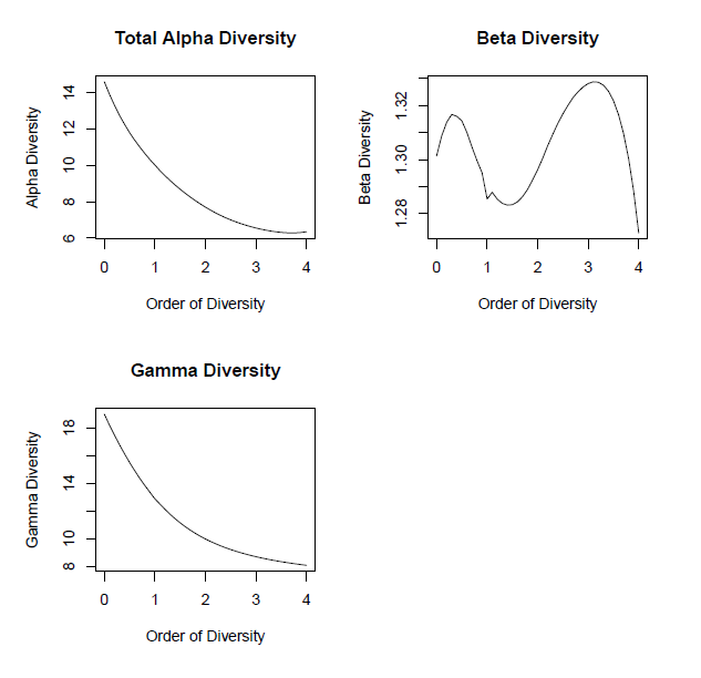
Recall the function DivProfiles we used at end of the previous session to plot Hill numbers. That function produces values of the α, β and γ diversity (and entropy) with order varying in the sequence we give it as input. For example
> divP.jv=DivProfile(seq(0,4,0.1),Meta.jv,Biased=FALSE)
and the plots for all the 3 profiles at once are obtained applying plot to the function's output
> plot(divP.jv)
Partizionamento delle diversitá
L'entropia γ di Tsallis e la diversitá γ possono essere facilmente partizionate nelle loro componenti α e β utilizzando le seguenti funzioni del pacchetto entropart:
- GammaEntropy() e GammaDiversity()
- AlphaEntropy() e AlphaDiversity()
- BetaEntropy() e BetaDiversity()
- DivPart é una funzione che combina tutte le funzioni precedenti
Si noti che tutte le funzioni α e β restituiscono liste con elementi di vettori:
> AlphaEntropy(Meta.jv,q=1) ##una lista con diverse informazioni
$MetaCommunity [1] "Meta.jv"
$Type
[1] "alpha"
$Order
[1] 1
$Correction
[1] "Best"
$Normalized
[1] TRUE
$Weights
| Allaine | Audeux | Clauge | Cuisance | Cusancin | Dessoubre | Doubs | Doulonnes | Drugeon | Furieuse | Lison | Loue |
| 0.03815114 | 0.02714600 | 0.09097579 | 0.05282465 | 0.02714600 | 0.03888481 | 0.22157007 | 0.02567865 | 0.07043287 | 0.04842260 | 0.05869406 | 0.30007337 |
| Allaine | Audeux | Clauge | Cuisance | Cusancin | Dessoubre | Doubs | Doulonnes | Drugeon | Furieuse | Lison | Loue |
| 2.122794 | 1.461630 | 2.632026 | 2.371961 | 1.474779 | 1.587543 | 2.465101 | 1.620635 | 2.235162 | 1.443209 | 1.994400 | 2.616050 |
$Total [1] 2.304366 attr(,"class") [1] "MCentropy"
> summary(AlphaEntropy(Meta.jv,q=1))
alpha Entropy of order 1 of MetaCommunity Meta.jv with correction: Best Entropy of communities:
| Allaine | Audeux | Clauge | Cuisance | Cusancin | Dessoubre | Doubs | Doulonnes | Drugeon | Furieuse | Lison | Loue |
| 2.122794 | 1.461630 | 2.632026 | 2.371961 | 1.474779 | 1.587543 | 2.465101 | 1.620635 | 2.235162 | 1.443209 | 1.994400 | 2.616050 |
Average entropy of the communities: [1] 2.304366
Si noti che
> GammaEntropy(Meta.jv,q=1,Correction="ChaoShen")
[1] 2.55195
restiituisce solo un valore ed lo stesso utilizzando la funzione Shannon(). Alcune differenze si osservano se si specifica l'opzione Correction="Best" nella funzione GammaEntrpy.> summary(BetaEntropy(Meta.jv,q=1))
beta Entropy of order 1 of MetaCommunity Meta.jv with correction: Best Entropy of communities:
| Allaine | Audeux | Clauge | Cuisance | Cusancin | Dessoubre | Doubs | Doulonnes | Drugeon | Furieuse | Lison | Loue |
| 0.42878299 | 0.56022760 | 0.35113958 | 0.08872304 | 0.65779757 | 0.58187935 | 0.11023280 | 0.97903461 | 0.46637253 | 0.50276549 | 0.33853664 | 0.15493055 |
Average entropy of the communities: [1] 0.2817997
Per realizzare grafici é piú opportuno assegnare l'output delle funzioni a degli oggetti:
> alpha.jv=AlphaEntropy(Meta.jv,q=1)
> beta.jv=BetaEntropy(Meta.jv,q=1)
> plot(alpha.jv,cex.names=0.5,main="allpha entropy of order 1")
> plot(beta.jv,cex.names=0.5,main="beta entropy of order 1")
Si noti gli effetti della correzione del bias sul valore della diversitá corrispondente all'entropia di Shannon:
> GammaDiversity(Meta.jv,q=1,Correction="Best")
[1] 12.87772
> GammaDiversity(Meta.jv,q=1,Correction="ChaoShen")
[1] 12.83211
Il partizionamento della diversitá senza correzione del bias é implementata nella funzione DivPart di default. Per applicare la correzione del bias é necessario impostare l'opzione Bias=FALSE e i defaults di correzione a "Best". Altre correzioni di bias possono essere selezionate tramite l'opzione Corrections. La sintassi é:
> DivPart(q=1,MC=Meta.jv,Bias=TRUE)
$MetaCommunity [1] "Meta.jv" $Order [1] 1 $Biased [1] TRUE $Correction [1] "Best" $Normalized [1] TRUE $TotalAlphaDiversity 12 [1] 9.471408 $TotalBetaDiversity [1] 1.354824 $GammaDiversity [1] 12.83209 $CommunityAlphaDiversities
| Allaine | Audeux | Clauge | Cuisance | Cusancin | Dessoubre | Doubs | Doulonnes | Drugeon | Furieuse | Lison | Loue |
| 7.240207 | 3.886486 | 12.740403 | 9.499748 | 3.861617 | 4.624712 | 11.340470 | 4.711500 | 8.804402 | 3.773609 | 6.725789 | 13.545080 |
$TotalAlphaEntropy [1] 2.248278 $TotalBetaEntropy [1] 0.3036712 $GammaEntropy [1] 2.551949 $CommunityAlphaEntropies
| Allaine | Audeux | Clauge | Cuisance | Cusancin | Dessoubre | Doubs | Doulonnes | Drugeon | Furieuse | Lison | Loue |
| 1.979650 | 1.357505 | 2.544778 | 2.251265 | 1.351086 | 1.531414 | 2.428378 | 1.550006 | 2.175252 | 1.328032 | 1.905949 | 2.606023 |
$CommunityBetaEntropies
| Allaine | Audeux | Clauge | Cuisance | Cusancin | Dessoubre | Doubs | Doulonnes | Drugeon | Furieuse | Lison | Loue |
| 0.4181963 | 0.5601920 | 0.3851946 | 0.1574901 | 0.7774108 | 0.6124040 | 0.1181721 | 1.0542939 | 0.4618816 | 0.6169071 | 0.3666474 | 0.1567946 |
attr(,"class") [1] "DivPart"
> DivPart(q=1,MC=Meta.jv,Bias=FALSE)
$MetaCommunity [1] "Meta.jv" $Order [1] 1 $Biased [1] FALSE $Correction [1] "Best" $Normalized [1] TRUE $TotalAlphaDiversity [1] 10.01783 $TotalBetaDiversity [1] 1.28548 $GammaDiversity [1] 12.87772 $CommunityAlphaDiversities
| Allaine | Audeux | Clauge | Cuisance | Cusancin | Dessoubre | Doubs | Doulonnes | Drugeon | Furieuse | Lison | Loue |
| 8.354445 | 4.312985 | 13.901902 | 10.718386 | 4.370071 | 4.891716 | 11.764667 | 5.056298 | 9.347999 | 4.234261 | 7.347792 | 13.681575 |
$TotalAlphaEntropy [1] 2.304366 $TotalBetaEntropy [1] 0.2511324 $GammaEntropy [1] 2.555498 $CommunityAlphaEntropies
| Allaine | Audeux | Clauge | Cuisance | Cusancin | Dessoubre | Doubs | Doulonnes | Drugeon | Furieuse | Lison | Loue |
| 2.122794 | 1.461630 | 2.632026 | 2.371961 | 1.474779 | 1.587543 | 2.465101 | 1.620635 | 2.235162 | 1.443209 | 1.994400 | 2.616050 |
$CommunityBetaEntropies [1] NA attr(,"class") [1] "DivPart"
Si osservi che se si applica una qualsiasi correzione, non vengono restituite Observe that when any correction is applied, no community beta entropies are returned. The returned object is of class "DivPart" and both summary and plot, have methods for it:
> divP.jv=DivPart(q=1,MC=Meta.jv,Bias=FALSE) > summary(divP.jv)
Il partizionamento della diversitá di ordine 1 della metacommunitá Meta.jv con la correzione: migliore diversitá α delle comunitá:
| Allaine | Audeux | Clauge | Cuisance | Cusancin | Dessoubre | Doubs | Doulonnes | Drugeon | Furieuse | Lison | Loue |
| 8.354445 | 4.312985 | 13.901902 | 10.718386 | 4.370071 | 4.891716 | 11.764667 | 5.056298 | 9.347999 | 4.234261 | 7.347792 | 13.681575 |
Total alpha diversity of the communities: [1] 10.01783 Beta diversity of the communities: [1] 1.28548 Gamma diversity of the metacommunity: [1] 12.87772
Nel grafico della partizione della diversitá della metacomunitá Meta.jv, il rettangolo di altezza 1 rappresenta la diversitá γ, uguale per circa 12 specie. Il rettangolo piú stretto e qullo piú alto hanno la stessa area: la dimensione orrizontale é la diversitá α (circa 10 specie effettive) e la sua altezza é la diversitá β (1.354 comunitá effettive).
> plot(divP.jv)
Per l'esempio di macroloire:
> plot(DivPart(q=1,MC=Meta.dat2))
In questo caso la diversitá γ é 8.66 (circa 9 specie effettive), il totale della diversitá α é 5.52 (circa 6 specie effettive) e la diversitá β é 1.57 (comunitá effettive). If we assume that community species counts are a realization of a multinomial probability distribution, they can be resampled from such distribution to obtain simulated entropies. The function DivEst estimates α, β and γ diversities and their confidence intervals obtained by simulation. It requires the order of the diversity (the corresponding Tsallis entropy), the meta-community, the number of simulations [2], the choice of a bias correction (TRUE or FALSE) and the name of the correction.
> divE.jv=DivEst(q=1,MC=Meta.jv,Simulations=500,Biased=FALSE,Correction="Best")
==============================================================================
> plot(divE.jv)
Recall the function DivProfiles we used at end of the previous session to plot Hill numbers. That function produces values of the α, β and γ diversity (and entropy) with order varying in the sequence we give it as input. For example
> divP.jv=DivProfile(seq(0,4,0.1),Meta.jv,Biased=FALSE)
and the plots for all the 3 profiles at once are obtained applying plot to the function's output
> plot(divP.jv)