Data Management and Biodiversity partitioning using the R package entropart - Gestione dati e partizione della biodiversità con il package entropart di R
| Site: | LifeWatch ERIC Training Platform |
| Course: | Introduction to partitioning and mixed models for biodiversity analysis in R |
| Book: | Data Management and Biodiversity partitioning using the R package entropart - Gestione dati e partizione della biodiversità con il package entropart di R |
| Printed by: | Guest user |
| Date: | Tuesday, 15 September 2026, 2:22 PM |
Description
Data Management and Biodiversity partitioning using the R package entropart - Gestione dati e partizione della biodiversità con il package entropart di R
Data Management
In the session Introduction to R we already saw how to read a text data file into R. We are now going to learn how to perform simple data manipulations in R. First of all we load into the workspace a dataset available package ade4, devoted to ecological analysis. By typing
> library(ade4)
> data(macroloire)
A total of 38 sites were surveyed along 800 km of the Loire River yielding 40 species of Trichoptera and Coleoptera sampled from riffle habitats. The river was divided into three regions according to ge- ology: granitic highlands (Region n.1), limestone lowlands (Region n.2) and granitic lowlands (Region n.3). This data set has been col- lected for analyzing changes in macroinvertebrate assemblages along the course of a large river. Four criteria are given here: variation in 1) species composition and relative abundance, 2) taxonomic composition, 3) Body Sizes, 4) Feeding habits.
Data are organized as elements of the macroloire list. In the faunistic table macroloire$fau , sites are on the columns and species on the rows. In the following examples interest is focused on communities defined by the grouping factor macroloire$envir$Morphoregion. Now in order to construct a faunistic table for the three regions, it is necessary to rearrange data so that abundances originally referred to monitoring stations are aggregated into the three commu- nities. First, in order to simplify the commands writing, extract the faunistic table and Morphoregion factor from the macroloire list:
> dat.1=macroloire$fau
> reg=macroloire$envir$Morphoregion
We want to sum abundances of each species recorded at sites, according to the region they belong to. For the first species in the macroloire faunistic table, i.e. the first row ofdat.1:
> tapply(t(dat.1[1,]),reg,sum)
| granitic highlands | granitic lowlands | limestone lowlands |
| 0 | 0 | 2 |
The function tapply allows to apply a function (in this case sum) to a vector according to a grouping factor [1]. Now we need to apply the same set of operations to each species, i.e. to each row of the faunistic table dat.1 Instead of manually doing this, it is easier to use a cycle. Cycles are useful whenever we need to replicate the same operation until a given condition is verified. The simplest and maybe most common situation is when we know exactly how many times an operation or a sequence of operations must be computed. The general structure of a cycle is for (k in 1:x){...}, where k is an index that will be incremented from 1 to x and the commands between curly brackets will be repeated x times.
We first create a new object with the same number of rows as dat.1 and 3 columns as communities in reg are 3. This object will become the new faunistic table.
> dat.2=matrix(0,nrow(dat.1),3)
The cycle implementing the construction of the faunistic table is:
> for(i in 1:nrow(dat.1)){
+ dat.2[i,]=tapply(t(dat.1[i,]),reg,sum)
+ }
> row.names(dat.2)=row.names(dat.1)
> colnames(dat.2)=levels(reg)
> dat.2=as.data.frame(dat.2)
The last three commands assign the species names to the rows of the new faunistic table, the names of the regions to its columns and transforms it into a data frame. As a first check we can verify it there are rare species in the dataset. This can be done by computing the total counts of the species (rows) in the dataset dat.2
> apply(dat.2,1,sum)
| E1 | E2 | E3 | E4 | E5 | E6 | E7 | E8 | E9 | E10 | E11 | E12 | E13 | |
| 2 | 7 | 4 | 1 | 40 | 4 | 8 | 134 | 29 | 75 | 2 | 8 | 13 | |
| E14 | E15 | E16 | E17 | E18 | E19 | E20 | E21 | E22 | E23 | E24 | E25 | E26 | |
| 24 | 4 | 1 | 1 | 90 | 2 | 29 | 115 | 77 | 1 | 130 | 259 | 1839 | |
| E27 | E28 | E29 | E30 | E31 | E32 | E33 | E34 | E35 | E36 | E37 | E38 | E39 | E40 |
| 10 | 1110 | 4 | 406 | 57 | 22 | 5 | 10 | 27 | 2 | 8 | 49 | 46 | 11 |
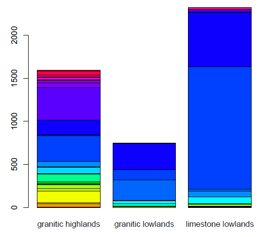
Several species are found only once or twice. Using the barplot function it is possible to visualize the distributions of the species in the three regions. The function requires an object of mode matrix as input that can be obtained calling the as.matrix() function in the the barplot command:
> barplot(as.matrix(dat.2),col=rainbow(40))
Gestione dei dati
Nella sezione "Introduzione a R" si é visto come importare un file dati di testo nell'ambiente di R. Ora si vedrÁ come effettuare delle semplici manipolazioni di dati in R. Per primo si carica nello spazio di lavoro un dataset disponibile nel package ade4, dedicato alle analisi ecologiche. Digitando
> library(ade4)
> data(macroloire)
Un totale di 38 siti sono stati censiti lungo 800 km del fiume della Loira, individuando 40 specie di Trichoptera e Coleoptera campionati dall'habitat che scorre. Il fiume é stato diviso in 3 regione in base alla sua geologia: gli altipiani granitici (Regione n.1), pianura calcarea (Regione n.2) e la pianura granitica (Regione n.3). Questo dataset é stato raccolto per analizzare cambiamenti dell'assembramento dei macroinvertebrati lungo il corso di un grande fiume. Sono dati 4 criteri: variazioni di 1) composizione delle specie e relativa abbondanza, 2) composizione tassonomica, 3) dimensioni corporali, 4) abitudini alimentari.
Nella lista macroloire i dati sono organizzati come elementi. Nella tabella faunistica macroloire$fau , i siti sono nelle colonne e le specie nelle righe. L'interesse del seguente esempio é focalizzato sulle comunitá definite da un fattore di raggruppamento macroloire$envir$Morphoregion. Per costruire una tabella faunistica per le tre regioni, é necessatrio riorganizzare i dati in modo che le abbondanze riferite alle stazioni di monitoraggio sono aggregate nelle tre comunitá. In modo da semplificare la digitazione dei comandi, si estraggono la tabella faunistica e il fattore Morphoregion dalla lista macroloire:
> dat.1=macroloire$fau
> reg=macroloire$envir$Morphoregion
Se si vogliono sommare le abbondanze di ogni specie registrate ai siti, tenendo conto della regione di appartenenza. Per la prima specie della tabella faunistica di macroloire, ossia il primo rigo di dat.1:
> tapply(t(dat.1[1,]),reg,sum)
| granitic highlands | granitic lowlands | limestone lowlands |
| 0 | 0 | 2 |
La funzione tapply permette di applicare un funzione (in questo caso sum) ad un vettore in base ad un fattore di raggruppamento [1]. Ora si applica lo stesso insieme di operazione ad orgni specie, ossia per ogni rigo della tabella faunistica dat.1. Invece di operare manualmente, é piú semplice utilizzare un ciclo. I cicli sono utili ogni qual volta si deve eseguire la stessa operazione finchè una determinata condizione non si verfichi. La piú semplice e piú comune situazione é quando si conosce il numero di volte che una operatzione o una sequenza di operazioni deve essere eseguita. La struttura generale di un ciclo é for (k in 1:x){...}, dove k é un indice che viene incrementato da 1 a x e i comandi fra parentesi graffe vengono ripetute x volte.
Per primo si crea un nuovo oggetto con lo stesso numero di rghi di dat.1 e 3 colonne siccome le comunitá in reg sono 3. Questo oggetto diventerá la nuova tabella faunistica.
> dat.2=matrix(0,nrow(dat.1),3)
Il ciclo che implementa la costruzione della tabella faunistica é:
> for(i in 1:nrow(dat.1)){
+ dat.2[i,]=tapply(t(dat.1[i,]),reg,sum)
+ }
> row.names(dat.2)=row.names(dat.1)
> colnames(dat.2)=levels(reg)
> dat.2=as.data.frame(dat.2)
Gli ultimi tre comandi assegnano i nomi delle specie alle righe della nuova tabella faunistica, i nome delle regioni alle sue colonne, trasformandola così in un data frame. Come primo controllo si puó verificare che vi sono specie rare presenti nel dataset. Ció si puó fare contando il numero di specie (righe) nel dataset dat.2
> apply(dat.2,1,sum)
| E1 | E2 | E3 | E4 | E5 | E6 | E7 | E8 | E9 | E10 | E11 | E12 | E13 | |
| 2 | 7 | 4 | 1 | 40 | 4 | 8 | 134 | 29 | 75 | 2 | 8 | 13 | |
| E14 | E15 | E16 | E17 | E18 | E19 | E20 | E21 | E22 | E23 | E24 | E25 | E26 | |
| 24 | 4 | 1 | 1 | 90 | 2 | 29 | 115 | 77 | 1 | 130 | 259 | 1839 | |
| E27 | E28 | E29 | E30 | E31 | E32 | E33 | E34 | E35 | E36 | E37 | E38 | E39 | E40 |
| 10 | 1110 | 4 | 406 | 57 | 22 | 5 | 10 | 27 | 2 | 8 | 49 | 46 | 11 |
Diverse specie sono state trovate solo una o due volte. Utilizzando la funzione barplot é possibile visualizzare la distribuzione delle specie nelle tre regioni. La funzione richiede un oggetto di modo matrix (matrixe) come dato di input e puó essere ottenuto invocando la funzione as.matrix() nel comando barplot:
> barplot(as.matrix(dat.2),col=rainbow(40))
The entropart package
To obtain information on the entire dataset it is useful to define a Meta-community as available in the entropart package.
> library(entropart)
Meta-communities can be built giving equal or different weights to the communities. Weights can be chosen arbitrarily but usually they are proportional to the number of individuals found in each community. Equally weighted communities are obtained as:
> Meta.dat2=MetaCommunity(dat.2,Weights=c(1,1,1))
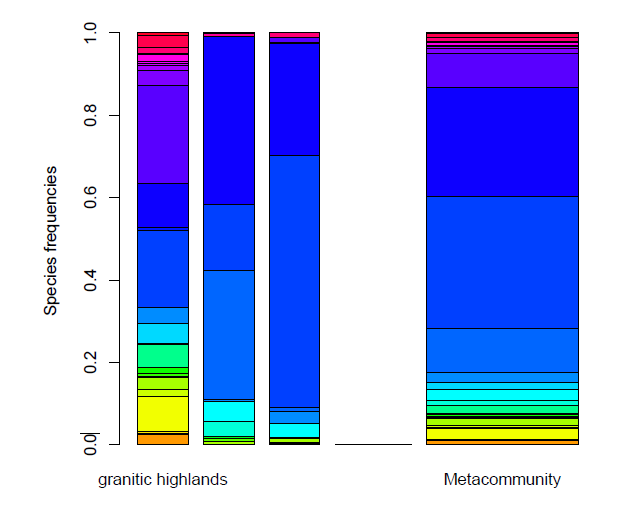
For objects of class MetaCommunity the summary and plot functions have specific methods:
> summary(Meta.dat2)
Meta-community (class 'MetaCommunity') made of 4785 individuals in 3 communities and 40 species.
Its sample coverage is 0.99914310220727
Community weights are:
| granitic highlands | granitic lowlands | limestone lowlands |
| 0.3333333 | 0.3333333 | 0.3333333 |
Community sample numbers of individuals are:
| granitic highlands | granitic lowlands | limestone lowlands |
| 1595 | 747 | 2324 |
Community sample coverages are:
| granitic highlands | granitic lowlands | limestone lowlands |
| 0.9981231 | 0.9973226 | 0.9987102 |
> plot(Meta.dat2,col=rainbow(40))
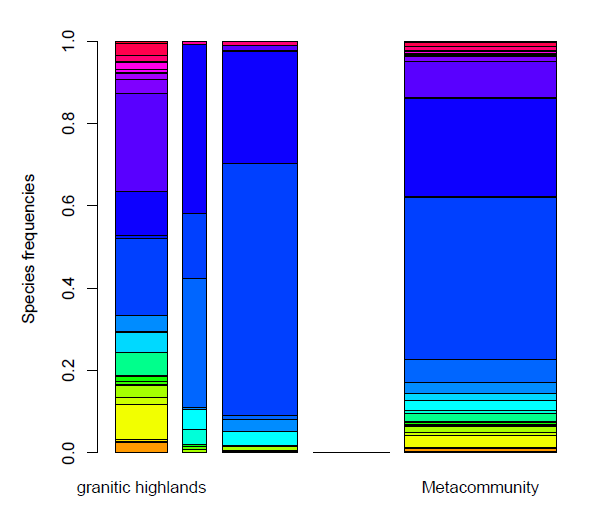
Notice the difference when the communities are weighted. Here we choose weights proportional to the number of individuals in each community:
> ww=c(1595,747,2324 )/(1595+747 +2324 ) > Meta.dat2a=MetaCommunity(dat.2,Weights=ww) > summary(Meta.dat2)
Meta-community (class 'MetaCommunity') made of 4666 individuals in 3 communities and 40 species.
Its sample coverage is 0.99914310220727
Community weights are:
| granitic highlands | granitic lowlands | limestone lowlands |
| 0.34183453 | 0.1600943 | 0.4980712 |
Community sample numbers of individuals are:
| granitic highlands | granitic lowlands | limestone lowlands |
| 1595 | 747 | 2324 |
Community sample coverages are:
| granitic highlands | granitic lowlands | limestone lowlands |
| 0.9981231 | 0.9973226 | 0.9987102 |
> plot(Meta.dat2,col=rainbow(40))
When meta-communities are built with this faunistic table a warning message is issued, as there is one species that is largely more abundant then the others in the third community (limestone lowlands), as can be seen by computing the community relative abundances:
> rela=dat.2[,3]/sum(dat.2[,3])
This unbalance creates a problem in the computation of bias corrections. Another interesting quantity that can be computed from the meta commu- nity object is the sample coverage, that is almost 1 in the current dataset for the three communities and for the metacommunity:
> Coverage(Ns=Meta.dat2$Ns)
[1] 0.9991627
In the macroloire list the names of the species are in the data frame element macroloire$labels. To associate species names to the above vector's elements consider that macroloire$labels is a data frame object and has to be addressed using the appropriate syntax:
> names(rela)=as.character(macroloire$labels[,1])
> rela
| Potamophilus acuminatus | Stenelmis canaliculata | Macronychus quadrituberculatus | Dupophilus brevis |
| 0.0008605852 | 0.0030120482 | 0.0017211704 | 0.0000000000 |
| Elmis aenea | Elmis maugetii | Elmis rioloides | Esolus angustatus |
| 0.0000000000 | 0.0000000000 | 0.0000000000 | 0.0000000000 |
| Esolus parallelepipedus | Esolus pygmaeus | Limnius perrisi | Limnius volckmari |
| 0.0004302926 | 0.0090361446 | 0.0000000000 | 0.0008605852 |
| Limnius opacus | Oulimnius troglodytes | Oulimnius tuberculatus | Platambus maculatus |
| 0.0004302926 | 0.0017211704 | 0.0000000000 | 0.0000000000 |
| Oreodytes sanmarkii | Oligoplectrum maculatum | Micrasema longulum | Ecnomus deceptor |
| 0.0000000000 | 0.0000000000 | 0.0000000000 | 0.0008605852 |
| Ecnomus tenellus | Glossosoma conformis | Agapetus delicatulus | Cheumatopsyche lepida |
| 0.0339931153 | 0.0000000000 | 0.0000000000 | 0.0275387263 |
| Hydropsyche bulgaromanorum | Hydropsyche contubernalis | Hydropsyche dinarica | Hydropsyche exocellata |
| 0.0107573150 | 0.6114457831 | 0.0000000000 | 0.2723752151 |
| Hydropsyche ornatula | Hydropsyche pellucidula | Hydropsyche siltalai | Allogamus auricollis |
| 0.0017211704 | 0.0116179002 | 0.0000000000 | 0.0000000000 |
| Chimarra marginata | Philopotamus montanus | Polycentropus flavomaculatus | Plectrocnemia geniculata |
| 0.0000000000 | 0.0000000000 | 0.0000000000 | 0.0000000000 |
| Neureclipsis bimaculata | Psychomyia pusilla | Rhyacophila praemorsa | Thremma gallicum |
| 0.0004302926 | 0.0111876076 | 0.0000000000 | 0.0000000000 |
The Hydropsyche contubernalis has a relative abundance of 0.611. Now consider a new faunistic table, namely the dataset jv73 of the package ade4:
This data set gives physical and physico-chemical variables, fish species, spatial coordinates about 92 sites. It is a list of 6 components:
- morpho is a data frame with 92 sites and 6 physical variables.
- phychi is a data frame with 92 sites and 12 physico-chemical variables.
- poi is a data frame with 92 sites and 19 fish species.
- xy is a data frame with 92 sites and 2 spatial coordinates.
- contour is a data frame for mapping.
- fac.riv is a factor distributing the 92 sites on 12 rivers.
As before the interest is in communities with spatial scale larger than the monitoring station. Communities are defined by each of 12 rivers, then it is necessary to create a new faunistic table with abundances (number of individuals here) aggregated by river. As in the previous example, it is convenient to extract the faunistic table from the list and then build the cycle:
> data(jv73)
> app=t(jv73$poi)
> jv73.fau=data.frame(matrix(0,nrow(app),ncol=12))
> for(i in 1:nrow(app)){
+ jv73.fau[i,]=tapply(t(app[i,]),jv73$fac.riv,sum)
+ }
> colnames(jv73.fau)=levels(jv73$fac.riv)
> row.names(jv73.fau)=row.names(app)
In the object jv73.fau the 12 communities are ready to be analyzed.
> apply(jv73.fau,2,sum)
| Allaine | Audeux | Clauge | Cuisance | Cusancin | Dessoubre |
| 52 | 37 | 124 | 72 | 37 | 53 |
| Doubs | Doulonnes | Drugeon | Furieuse | Lison | Loue |
| 302 | 35 | 96 | 66 | 80 | 409 |
Notice that very different abundances are observed in the 12 communities:
> ww.jv=apply(jv73.fau,2,sum)/(sum(apply(jv73.fau,2,sum) ))
This suggests the construction of a weighted meta-community, obtained with following syntax:
> Meta.jv=MetaCommunity(jv73.fau,Weights=ww.jv)
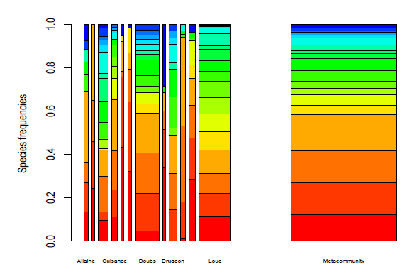
To plot the meta-community giving one color to each species it is convenient to build a color palette. The function colorRampPalette allows to build the desired graduated color scale:
> plot(Meta.jv,col=colorRampPalette(c("red","yellow","green","cyan","blue"))(19), + cex.names=0.5)
To get familiar with the entropart package it is useful to experiment with some of its functions. To compute Tsallis entropies there is the function with the same name
> Tsallis(Ps=Meta.jv$Ps,q=1)
[1] 2.551949
Same as:
> Shannon(Ps=Meta.jv$Ps)
[1] 2.551949
To apply the bias correction write:
> bcTsallis(Ns=Meta.jv$Ns,q=1)
[1] 2.555498
> bcShannon(Ns=Meta.jv$Ns)
[1] 2.555498
Notice that no differences are found when the coverage is almost 1, i.e no singletons are found in the faunistic table
> Coverage(Ns=Meta.jv$Ns)
[1] 1
To compute the Hill numbers corresponding to the Simpson index (Tsallis entropy with q = 2 or also the Gini's index introduced in 1920's to study income distributions) write:
> expq(Tsallis(Ps=Meta.jv$Ps,q=2),q=2)
[1] 9.906675
that is the same as
> Diversity(Ps=Meta.jv$Ps,q=2)
[1] 9.906675
To apply the bias correction to the diversity measure:
> bcDiversity(Ns=Meta.jv$Ns,q=2)
[1] 9.979207
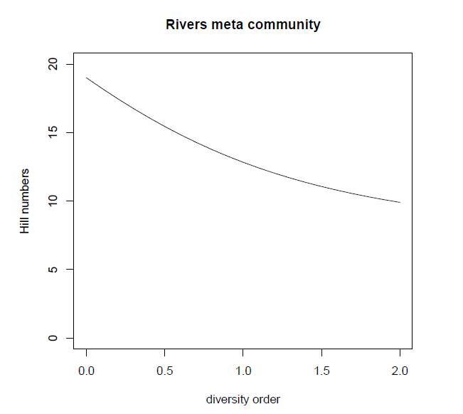
The corrected diversities can be interpreted extending the idea of effective number of species, or Hill numbers. They can be examined with different types of plots.
The schematic procedure is:
- prepare a vector with the diversities order
- compute the diversity profile using DivProfile
- extract the gamma diversity from the diversity profile object
- plot the gamma diversity vs the diversities order
> qq=seq(0,2,by=0.1)
> dd=DivProfile(qq,Meta.jv)
> names(dd)
| [1] | "MetaCommunity" | "Order" | "Biased" | "Correction" | "Normalized" |
| [6] | "TotalAlphaDiversity" | "TotalBetaDiversity" | "GammaDiversity" | "TotalAlphaEntropy" | "TotalBetaEntropy" |
| [11] | "GammaEntropy" |
> plotHn=dd$GammaDiversity
> plot(qq,plotHn,type="l",ylim=c(0,20),xlab="diversity order",
+ylab="Hill numbers",main="Rivers meta community")
Il pacchetto entropart
Per ottenere informazioni sull'intero data set é utile definire una meta-comunitá come "disponibile" nel pacchetto entropart.
> library(entropart)
Meta-comunitá possono essere create dando pesi uguali o differenti alle comunitá. I pesi possono essere scelti arbitrariamente, ma in genere sono proporzionali al numero di esemplari popolanti la singola comunitá. Comunitá con pesi uguali sono ottenuti come:
> Meta.dat2=MetaCommunity(dat.2,Weights=c(1,1,1))
Per oggetti della classe MetaComunity le funzioni summary e plot hanno metodi specifici:
> summary(Meta.dat2)
Meta-community (class 'MetaCommunity') made of 4785 individuals in 3 communities and 40 species.
Its sample coverage is 0.99914310220727
Community weights are:
| granitic highlands | granitic lowlands | limestone lowlands |
| 0.3333333 | 0.3333333 | 0.3333333 |
Community sample numbers of individuals are:
| granitic highlands | granitic lowlands | limestone lowlands |
| 1595 | 747 | 2324 |
Community sample coverages are:
| granitic highlands | granitic lowlands | limestone lowlands |
| 0.9981231 | 0.9973226 | 0.9987102 |
> plot(Meta.dat2,col=rainbow(40))
Notice the difference when the communities are weighted. Here we choose weights proportional to the number of individuals in each community:
> ww=c(1595,747,2324 )/(1595+747 +2324 ) > Meta.dat2a=MetaCommunity(dat.2,Weights=ww) > summary(Meta.dat2)
Meta-community (class 'MetaCommunity') made of 4666 individuals in 3 communities and 40 species.
Its sample coverage is 0.99914310220727
Community weights are:
| granitic highlands | granitic lowlands | limestone lowlands |
| 0.34183453 | 0.1600943 | 0.4980712 |
Community sample numbers of individuals are:
| granitic highlands | granitic lowlands | limestone lowlands |
| 1595 | 747 | 2324 |
Community sample coverages are:
| granitic highlands | granitic lowlands | limestone lowlands |
| 0.9981231 | 0.9973226 | 0.9987102 |
> plot(Meta.dat2,col=rainbow(40))
Quando sono create meta-comunitá con questa tabella faunistica, viene lanciato un messaggio di avvertimento (warning), siccome una specie é molto piú abbondante che le altre nella terza comunitá (bassopiano calcareo), come si puó vedere calcolando le abbondanze relative della comunitá:
> rela=dat.2[,3]/sum(dat.2[,3])
Questo sbilanciamento crea problemi nel calcolo delle correzioni degli errori (bias). Un altro interessante valore che puó essere calcolato dall'oggetto meta-comunitá é la copertura campionaria, che é pressoché 1 nel dataset corrente per le tre comunitá e per la metacomunitá:
> Coverage(Ns=Meta.dat2$Ns)
[1] 0.9991627
Nella lista macroloire i nome delle specie sono indicate nell'elemento del dataframe macroloire$labels. Per associare i nomi delle specie agli elementi del vettore precedente si consideri che macroloire$labels é un oggetto del dataframe e deve essere indirizzato con un adeguata sintassi:
> names(rela)=as.character(macroloire$labels[,1])
> rela
| Potamophilus acuminatus | Stenelmis canaliculata | Macronychus quadrituberculatus | Dupophilus brevis |
| 0.0008605852 | 0.0030120482 | 0.0017211704 | 0.0000000000 |
| Elmis aenea | Elmis maugetii | Elmis rioloides | Esolus angustatus |
| 0.0000000000 | 0.0000000000 | 0.0000000000 | 0.0000000000 |
| Esolus parallelepipedus | Esolus pygmaeus | Limnius perrisi | Limnius volckmari |
| 0.0004302926 | 0.0090361446 | 0.0000000000 | 0.0008605852 |
| Limnius opacus | Oulimnius troglodytes | Oulimnius tuberculatus | Platambus maculatus |
| 0.0004302926 | 0.0017211704 | 0.0000000000 | 0.0000000000 |
| Oreodytes sanmarkii | Oligoplectrum maculatum | Micrasema longulum | Ecnomus deceptor |
| 0.0000000000 | 0.0000000000 | 0.0000000000 | 0.0008605852 |
| Ecnomus tenellus | Glossosoma conformis | Agapetus delicatulus | Cheumatopsyche lepida |
| 0.0339931153 | 0.0000000000 | 0.0000000000 | 0.0275387263 |
| Hydropsyche bulgaromanorum | Hydropsyche contubernalis | Hydropsyche dinarica | Hydropsyche exocellata |
| 0.0107573150 | 0.6114457831 | 0.0000000000 | 0.2723752151 |
| Hydropsyche ornatula | Hydropsyche pellucidula | Hydropsyche siltalai | Allogamus auricollis |
| 0.0017211704 | 0.0116179002 | 0.0000000000 | 0.0000000000 |
| Chimarra marginata | Philopotamus montanus | Polycentropus flavomaculatus | Plectrocnemia geniculata |
| 0.0000000000 | 0.0000000000 | 0.0000000000 | 0.0000000000 |
| Neureclipsis bimaculata | Psychomyia pusilla | Rhyacophila praemorsa | Thremma gallicum |
| 0.0004302926 | 0.0111876076 | 0.0000000000 | 0.0000000000 |
La Hydropsyche contubernalis ha una abondanza relativa di 0.611. Si consideri una nuova tabella faunistica, ossia il dataset jv73 del pacchetto ade4:
Questo dataset fornisce viariabili fisiche e fisico-chimiche, specie di pesci, coordianate spaziale di circa 92 siti. É una lista di 6 componenti:
- morpho é un dataframe con 92 siti e 6 variabili fisiche.
- phychi é un dataframe con 92 siti e 12 variabili fisico-chimiche.
- poi é un dataframe con 92 siti e 19 specie di pesci.
- xy é un dataframe con 92 siti e 2 coordinate spaziali.
- contour é un dataframe per la mappatura.
- fac.riv é un fattore che distribuisce i 92 siti su 12 fiumi.
Siccome, come prima, l'interesse é per le comunitá con una scala spaziale maggiore di una stazione di monitoraggio. Comunitá sono definite da ogniuno dei 12 fiumi, quindi é necessario creare una nuova tabella faunistica con le abbondanze (numero di esemplari) aggragati dal fiume. Come nell'esempio precedente, é opportuno estrarre la tabella faunistica dalla lista e poi creare il ciclo:
> data(jv73)
> app=t(jv73$poi)
> jv73.fau=data.frame(matrix(0,nrow(app),ncol=12))
> for(i in 1:nrow(app)){
+ jv73.fau[i,]=tapply(t(app[i,]),jv73$fac.riv,sum)
+ }
> colnames(jv73.fau)=levels(jv73$fac.riv)
> row.names(jv73.fau)=row.names(app)
Nell'oggetto jv73.fau le 12 comunitá sono pronte ad essere analizzate.
> apply(jv73.fau,2,sum)
| Allaine | Audeux | Clauge | Cuisance | Cusancin | Dessoubre |
| 52 | 37 | 124 | 72 | 37 | 53 |
| Doubs | Doulonnes | Drugeon | Furieuse | Lison | Loue |
| 302 | 35 | 96 | 66 | 80 | 409 |
Si osservano abbondanze molto differenti nelle 12 comunitá:
> ww.jv=apply(jv73.fau,2,sum)/(sum(apply(jv73.fau,2,sum) ))
Questo suggerisce la costruzione di una meta-comunitá ponderata, ottenuta con la seguente sintassi:
> Meta.jv=MetaCommunity(jv73.fau,Weights=ww.jv)
Per disegnare una meta-comunitá specificando un colore per ogni specie é opportuno creare una palette di colori. La funzione colorRampPalette consente di realizzare la scala graduata di colori desiderata:
> plot(Meta.jv,col=colorRampPalette(c("red","yellow","green","cyan","blue"))(19), + cex.names=0.5)
Per familiarizzare con il pacchetto entropart é utile sperimentare con alcune delle sue funzioni. Per calcolare le entropie di Tsallis esiste una funzione che ha lo stesso nome:
> Tsallis(Ps=Meta.jv$Ps,q=1)
[1] 2.551949
Come anche:
> Shannon(Ps=Meta.jv$Ps)
[1] 2.551949
Per applicare la correzione del bias si scriva:
> bcTsallis(Ns=Meta.jv$Ns,q=1)
[1] 2.555498
> bcShannon(Ns=Meta.jv$Ns)
[1] 2.555498
Si noti che non ci sono differenze se la copertura é ciraca 1, ossia non vi sono esemplari singoli nella tabella faunistica:
> Coverage(Ns=Meta.jv$Ns)
[1] 1
Per calcolare i numeri di Hill corrispondenti all'indice di Simpson (entropia di Tsallis con q=2 oppure l'indice di Gini introdotto negli anni '20 per studiare la distribuzione dei reditti) si scriva:
> expq(Tsallis(Ps=Meta.jv$Ps,q=2),q=2)
[1] 9.906675
che é lo stessi a
> Diversity(Ps=Meta.jv$Ps,q=2)
[1] 9.906675
Per eseguire la correzione del bias al valore della diversitá:
> bcDiversity(Ns=Meta.jv$Ns,q=2)
[1] 9.979207
Le diversitá corrette posssono essere interpretate esetendendo il concetto di numero di specie effettive, o numeri di Hill: Possono essere esaminate con diversi tipi di grafici.
Lo schema delle procedure é:
- preparare un vettore con l'ordine delle diversitá
- calcolare il profilo della diversitá usando DivProfile
- estrarre la diversitá gamma dall'oggetto profilo di divesitá(diversity profile object)
- disegnare la difersitá gamma relazionata all'ordine (grado) di diversitá
> qq=seq(0,2,by=0.1)
> dd=DivProfile(qq,Meta.jv)
> names(dd)
| [1] | "MetaCommunity" | "Order" | "Biased" | "Correction" | "Normalized" |
| [6] | "TotalAlphaDiversity" | "TotalBetaDiversity" | "GammaDiversity" | "TotalAlphaEntropy" | "TotalBetaEntropy" |
| [11] | "GammaEntropy" |
> plotHn=dd$GammaDiversity
> plot(qq,plotHn,type="l",ylim=c(0,20),xlab="diversity order",
+ylab="Hill numbers",main="Rivers meta community")
Diversity partitioning
Tsallis γ entropies and diversity are easily partitioned into α and β components using the entropart package functions:- GammaEntropy() and GammaDiversity()
- AlphaEntropy() and AlphaDiversity()
- BetaEntropy() and BetaDiversity()
- DivPart is a function combining all the above functions
Notice that all α and β functions return lists with vector elements:
> AlphaEntropy(Meta.jv,q=1) ##a list with several information
$MetaCommunity [1] "Meta.jv"
$Type
[1] "alpha"
$Order
[1] 1
$Correction
[1] "Best"
$Normalized
[1] TRUE
$Weights
| Allaine | Audeux | Clauge | Cuisance | Cusancin | Dessoubre | Doubs | Doulonnes | Drugeon | Furieuse | Lison | Loue |
| 0.03815114 | 0.02714600 | 0.09097579 | 0.05282465 | 0.02714600 | 0.03888481 | 0.22157007 | 0.02567865 | 0.07043287 | 0.04842260 | 0.05869406 | 0.30007337 |
| Allaine | Audeux | Clauge | Cuisance | Cusancin | Dessoubre | Doubs | Doulonnes | Drugeon | Furieuse | Lison | Loue |
| 2.122794 | 1.461630 | 2.632026 | 2.371961 | 1.474779 | 1.587543 | 2.465101 | 1.620635 | 2.235162 | 1.443209 | 1.994400 | 2.616050 |
$Total [1] 2.304366 attr(,"class") [1] "MCentropy"
> summary(AlphaEntropy(Meta.jv,q=1))
alpha Entropy of order 1 of MetaCommunity Meta.jv with correction: Best Entropy of communities:
| Allaine | Audeux | Clauge | Cuisance | Cusancin | Dessoubre | Doubs | Doulonnes | Drugeon | Furieuse | Lison | Loue |
| 2.122794 | 1.461630 | 2.632026 | 2.371961 | 1.474779 | 1.587543 | 2.465101 | 1.620635 | 2.235162 | 1.443209 | 1.994400 | 2.616050 |
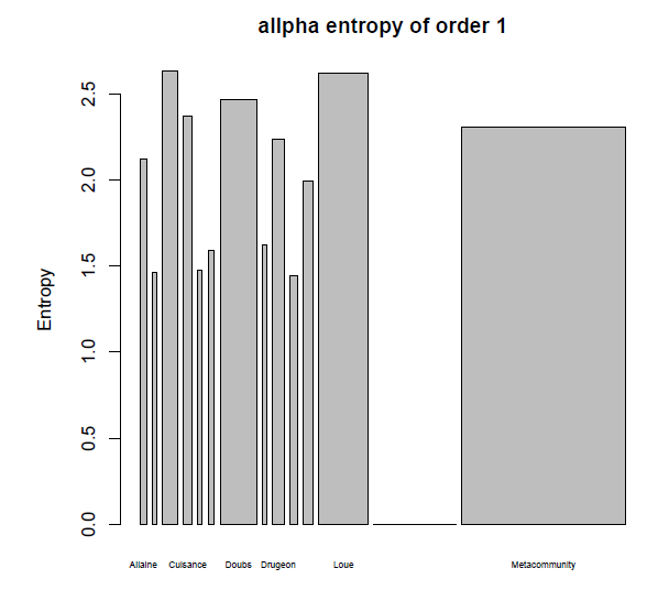
Average entropy of the communities: [1] 2.304366
Notice that
> GammaEntropy(Meta.jv,q=1,Correction="ChaoShen")
[1] 2.55195
returns only one value and the same value obtained running the Shannon() function. Some difference is observed if the option Correction="Best" is specified in the GammaEntropy function.> summary(BetaEntropy(Meta.jv,q=1))
beta Entropy of order 1 of MetaCommunity Meta.jv with correction: Best Entropy of communities:
| Allaine | Audeux | Clauge | Cuisance | Cusancin | Dessoubre | Doubs | Doulonnes | Drugeon | Furieuse | Lison | Loue |
| 0.42878299 | 0.56022760 | 0.35113958 | 0.08872304 | 0.65779757 | 0.58187935 | 0.11023280 | 0.97903461 | 0.46637253 | 0.50276549 | 0.33853664 | 0.15493055 |
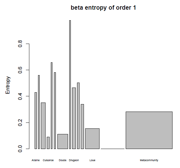
Average entropy of the communities: [1] 0.2817997
To build plots it is more convenient to assign functions outputs to objects:
> alpha.jv=AlphaEntropy(Meta.jv,q=1)
> beta.jv=BetaEntropy(Meta.jv,q=1)
> plot(alpha.jv,cex.names=0.5,main="allpha entropy of order 1")
> plot(beta.jv,cex.names=0.5,main="beta entropy of order 1")
Notice the effects of Bias correction on the diversity measure corresponding to the Shannon entropy:
> GammaDiversity(Meta.jv,q=1,Correction="Best")
[1] 12.87772
> GammaDiversity(Meta.jv,q=1,Correction="ChaoShen")
[1] 12.83211
Diversity partitioning is implement in the function DivPart with no bias correction chosen by default. The option Bias=F has to be set in the function to apply a correction and defaults to the \Best" correction. Other bias corrections can be selected by the Correction option. The syntax is:
> DivPart(q=1,MC=Meta.jv,Bias=TRUE)
$MetaCommunity [1] "Meta.jv" $Order [1] 1 $Biased [1] TRUE $Correction [1] "Best" $Normalized [1] TRUE $TotalAlphaDiversity 12 [1] 9.471408 $TotalBetaDiversity [1] 1.354824 $GammaDiversity [1] 12.83209 $CommunityAlphaDiversities
| Allaine | Audeux | Clauge | Cuisance | Cusancin | Dessoubre | Doubs | Doulonnes | Drugeon | Furieuse | Lison | Loue |
| 7.240207 | 3.886486 | 12.740403 | 9.499748 | 3.861617 | 4.624712 | 11.340470 | 4.711500 | 8.804402 | 3.773609 | 6.725789 | 13.545080 |
$TotalAlphaEntropy [1] 2.248278 $TotalBetaEntropy [1] 0.3036712 $GammaEntropy [1] 2.551949 $CommunityAlphaEntropies
| Allaine | Audeux | Clauge | Cuisance | Cusancin | Dessoubre | Doubs | Doulonnes | Drugeon | Furieuse | Lison | Loue |
| 1.979650 | 1.357505 | 2.544778 | 2.251265 | 1.351086 | 1.531414 | 2.428378 | 1.550006 | 2.175252 | 1.328032 | 1.905949 | 2.606023 |
$CommunityBetaEntropies
| Allaine | Audeux | Clauge | Cuisance | Cusancin | Dessoubre | Doubs | Doulonnes | Drugeon | Furieuse | Lison | Loue |
| 0.4181963 | 0.5601920 | 0.3851946 | 0.1574901 | 0.7774108 | 0.6124040 | 0.1181721 | 1.0542939 | 0.4618816 | 0.6169071 | 0.3666474 | 0.1567946 |
attr(,"class") [1] "DivPart"
> DivPart(q=1,MC=Meta.jv,Bias=FALSE)
$MetaCommunity [1] "Meta.jv" $Order [1] 1 $Biased [1] FALSE $Correction [1] "Best" $Normalized [1] TRUE $TotalAlphaDiversity [1] 10.01783 $TotalBetaDiversity [1] 1.28548 $GammaDiversity [1] 12.87772 $CommunityAlphaDiversities
| Allaine | Audeux | Clauge | Cuisance | Cusancin | Dessoubre | Doubs | Doulonnes | Drugeon | Furieuse | Lison | Loue |
| 8.354445 | 4.312985 | 13.901902 | 10.718386 | 4.370071 | 4.891716 | 11.764667 | 5.056298 | 9.347999 | 4.234261 | 7.347792 | 13.681575 |
$TotalAlphaEntropy [1] 2.304366 $TotalBetaEntropy [1] 0.2511324 $GammaEntropy [1] 2.555498 $CommunityAlphaEntropies
| Allaine | Audeux | Clauge | Cuisance | Cusancin | Dessoubre | Doubs | Doulonnes | Drugeon | Furieuse | Lison | Loue |
| 2.122794 | 1.461630 | 2.632026 | 2.371961 | 1.474779 | 1.587543 | 2.465101 | 1.620635 | 2.235162 | 1.443209 | 1.994400 | 2.616050 |
$CommunityBetaEntropies [1] NA attr(,"class") [1] "DivPart"
Observe that when any correction is applied, no community beta entropies are returned. The returned object is of class \DivPart" and both summary and plot, have methods for it:
> divP.jv=DivPart(q=1,MC=Meta.jv,Bias=FALSE) > summary(divP.jv)
Diversity partitioning of order 1 of MetaCommunity Meta.jv with correction: Best Alpha diversity of communities:
| Allaine | Audeux | Clauge | Cuisance | Cusancin | Dessoubre | Doubs | Doulonnes | Drugeon | Furieuse | Lison | Loue |
| 8.354445 | 4.312985 | 13.901902 | 10.718386 | 4.370071 | 4.891716 | 11.764667 | 5.056298 | 9.347999 | 4.234261 | 7.347792 | 13.681575 |
Total alpha diversity of the communities: [1] 10.01783 Beta diversity of the communities: [1] 1.28548 Gamma diversity of the metacommunity: [1] 12.87772
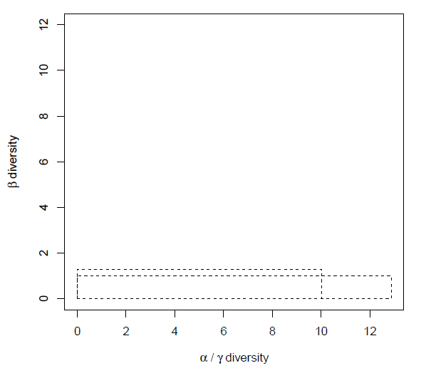
In the plot of the diversity partition of the meta-community Meta.jv, the long rectangle of height 1 represents γ diversity, equal to about 12 effective species. The narrower and higher rectangle has the same area: its horizontal size is α diversity (about 10 effective species) and its height is β diversity (1.354 effective communities).
> plot(divP.jv)
For the macroloire example we have:
> plot(DivPart(q=1,MC=Meta.dat2))
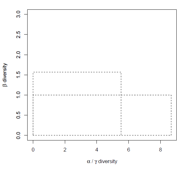
Here the γ-diversity is 8.66 (about 9 effective species), the total α-diversity is 5.52 (about 6 effective species) and the β-diversity is 1.57 (effective communities). If we assume that community species counts are a realization of a multinomial probability distribution, they can be resampled from such distribution to obtain simulated entropies. The function DivEst estimates α, β and γ diversities and their confidence intervals obtained by simulation. It requires the order of the diversity (the corresponding Tsallis entropy), the meta-community, the number of simulations [2], the choice of a bias correction (TRUE or FALSE) and the name of the correction.
> divE.jv=DivEst(q=1,MC=Meta.jv,Simulations=500,Biased=FALSE,Correction="Best")
==============================================================================
> plot(divE.jv)
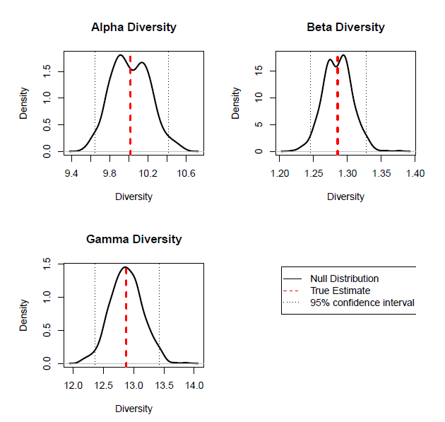
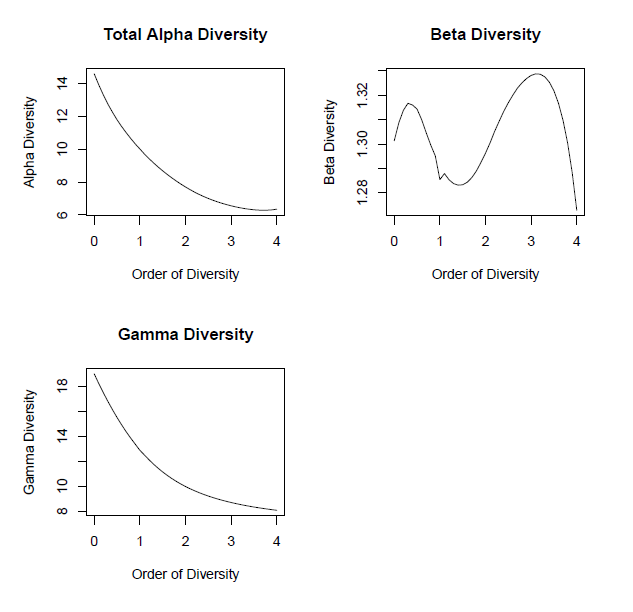
Recall the function DivProfiles we used at end of the previous session to plot Hill numbers. That function produces values of the α, β and γ diversity (and entropy) with order varying in the sequence we give it as input. For example
> divP.jv=DivProfile(seq(0,4,0.1),Meta.jv,Biased=FALSE)
and the plots for all the 3 profiles at once are obtained applying plot to the function's output
> plot(divP.jv)
Partizionamento delle diversitá
L'entropia γ di Tsallis e la diversitá γ possono essere facilmente partizionate nelle loro componenti α e β utilizzando le seguenti funzioni del pacchetto entropart:
- GammaEntropy() e GammaDiversity()
- AlphaEntropy() e AlphaDiversity()
- BetaEntropy() e BetaDiversity()
- DivPart é una funzione che combina tutte le funzioni precedenti
Si noti che tutte le funzioni α e β restituiscono liste con elementi di vettori:
> AlphaEntropy(Meta.jv,q=1) ##una lista con diverse informazioni
$MetaCommunity [1] "Meta.jv"
$Type
[1] "alpha"
$Order
[1] 1
$Correction
[1] "Best"
$Normalized
[1] TRUE
$Weights
| Allaine | Audeux | Clauge | Cuisance | Cusancin | Dessoubre | Doubs | Doulonnes | Drugeon | Furieuse | Lison | Loue |
| 0.03815114 | 0.02714600 | 0.09097579 | 0.05282465 | 0.02714600 | 0.03888481 | 0.22157007 | 0.02567865 | 0.07043287 | 0.04842260 | 0.05869406 | 0.30007337 |
| Allaine | Audeux | Clauge | Cuisance | Cusancin | Dessoubre | Doubs | Doulonnes | Drugeon | Furieuse | Lison | Loue |
| 2.122794 | 1.461630 | 2.632026 | 2.371961 | 1.474779 | 1.587543 | 2.465101 | 1.620635 | 2.235162 | 1.443209 | 1.994400 | 2.616050 |
$Total [1] 2.304366 attr(,"class") [1] "MCentropy"
> summary(AlphaEntropy(Meta.jv,q=1))
alpha Entropy of order 1 of MetaCommunity Meta.jv with correction: Best Entropy of communities:
| Allaine | Audeux | Clauge | Cuisance | Cusancin | Dessoubre | Doubs | Doulonnes | Drugeon | Furieuse | Lison | Loue |
| 2.122794 | 1.461630 | 2.632026 | 2.371961 | 1.474779 | 1.587543 | 2.465101 | 1.620635 | 2.235162 | 1.443209 | 1.994400 | 2.616050 |
Average entropy of the communities: [1] 2.304366
Si noti che
> GammaEntropy(Meta.jv,q=1,Correction="ChaoShen")
[1] 2.55195
restiituisce solo un valore ed lo stesso utilizzando la funzione Shannon(). Alcune differenze si osservano se si specifica l'opzione Correction="Best" nella funzione GammaEntrpy.> summary(BetaEntropy(Meta.jv,q=1))
beta Entropy of order 1 of MetaCommunity Meta.jv with correction: Best Entropy of communities:
| Allaine | Audeux | Clauge | Cuisance | Cusancin | Dessoubre | Doubs | Doulonnes | Drugeon | Furieuse | Lison | Loue |
| 0.42878299 | 0.56022760 | 0.35113958 | 0.08872304 | 0.65779757 | 0.58187935 | 0.11023280 | 0.97903461 | 0.46637253 | 0.50276549 | 0.33853664 | 0.15493055 |
Average entropy of the communities: [1] 0.2817997
Per realizzare grafici é piú opportuno assegnare l'output delle funzioni a degli oggetti:
> alpha.jv=AlphaEntropy(Meta.jv,q=1)
> beta.jv=BetaEntropy(Meta.jv,q=1)
> plot(alpha.jv,cex.names=0.5,main="allpha entropy of order 1")
> plot(beta.jv,cex.names=0.5,main="beta entropy of order 1")
Si noti gli effetti della correzione del bias sul valore della diversitá corrispondente all'entropia di Shannon:
> GammaDiversity(Meta.jv,q=1,Correction="Best")
[1] 12.87772
> GammaDiversity(Meta.jv,q=1,Correction="ChaoShen")
[1] 12.83211
Il partizionamento della diversitá senza correzione del bias é implementata nella funzione DivPart di default. Per applicare la correzione del bias é necessario impostare l'opzione Bias=FALSE e i defaults di correzione a "Best". Altre correzioni di bias possono essere selezionate tramite l'opzione Corrections. La sintassi é:
> DivPart(q=1,MC=Meta.jv,Bias=TRUE)
$MetaCommunity [1] "Meta.jv" $Order [1] 1 $Biased [1] TRUE $Correction [1] "Best" $Normalized [1] TRUE $TotalAlphaDiversity 12 [1] 9.471408 $TotalBetaDiversity [1] 1.354824 $GammaDiversity [1] 12.83209 $CommunityAlphaDiversities
| Allaine | Audeux | Clauge | Cuisance | Cusancin | Dessoubre | Doubs | Doulonnes | Drugeon | Furieuse | Lison | Loue |
| 7.240207 | 3.886486 | 12.740403 | 9.499748 | 3.861617 | 4.624712 | 11.340470 | 4.711500 | 8.804402 | 3.773609 | 6.725789 | 13.545080 |
$TotalAlphaEntropy [1] 2.248278 $TotalBetaEntropy [1] 0.3036712 $GammaEntropy [1] 2.551949 $CommunityAlphaEntropies
| Allaine | Audeux | Clauge | Cuisance | Cusancin | Dessoubre | Doubs | Doulonnes | Drugeon | Furieuse | Lison | Loue |
| 1.979650 | 1.357505 | 2.544778 | 2.251265 | 1.351086 | 1.531414 | 2.428378 | 1.550006 | 2.175252 | 1.328032 | 1.905949 | 2.606023 |
$CommunityBetaEntropies
| Allaine | Audeux | Clauge | Cuisance | Cusancin | Dessoubre | Doubs | Doulonnes | Drugeon | Furieuse | Lison | Loue |
| 0.4181963 | 0.5601920 | 0.3851946 | 0.1574901 | 0.7774108 | 0.6124040 | 0.1181721 | 1.0542939 | 0.4618816 | 0.6169071 | 0.3666474 | 0.1567946 |
attr(,"class") [1] "DivPart"
> DivPart(q=1,MC=Meta.jv,Bias=FALSE)
$MetaCommunity [1] "Meta.jv" $Order [1] 1 $Biased [1] FALSE $Correction [1] "Best" $Normalized [1] TRUE $TotalAlphaDiversity [1] 10.01783 $TotalBetaDiversity [1] 1.28548 $GammaDiversity [1] 12.87772 $CommunityAlphaDiversities
| Allaine | Audeux | Clauge | Cuisance | Cusancin | Dessoubre | Doubs | Doulonnes | Drugeon | Furieuse | Lison | Loue |
| 8.354445 | 4.312985 | 13.901902 | 10.718386 | 4.370071 | 4.891716 | 11.764667 | 5.056298 | 9.347999 | 4.234261 | 7.347792 | 13.681575 |
$TotalAlphaEntropy [1] 2.304366 $TotalBetaEntropy [1] 0.2511324 $GammaEntropy [1] 2.555498 $CommunityAlphaEntropies
| Allaine | Audeux | Clauge | Cuisance | Cusancin | Dessoubre | Doubs | Doulonnes | Drugeon | Furieuse | Lison | Loue |
| 2.122794 | 1.461630 | 2.632026 | 2.371961 | 1.474779 | 1.587543 | 2.465101 | 1.620635 | 2.235162 | 1.443209 | 1.994400 | 2.616050 |
$CommunityBetaEntropies [1] NA attr(,"class") [1] "DivPart"
Si osservi che se si applica una qualsiasi correzione, non vengono restituite Observe that when any correction is applied, no community beta entropies are returned. The returned object is of class "DivPart" and both summary and plot, have methods for it:
> divP.jv=DivPart(q=1,MC=Meta.jv,Bias=FALSE) > summary(divP.jv)
Il partizionamento della diversitá di ordine 1 della metacommunitá Meta.jv con la correzione: migliore diversitá α delle comunitá:
| Allaine | Audeux | Clauge | Cuisance | Cusancin | Dessoubre | Doubs | Doulonnes | Drugeon | Furieuse | Lison | Loue |
| 8.354445 | 4.312985 | 13.901902 | 10.718386 | 4.370071 | 4.891716 | 11.764667 | 5.056298 | 9.347999 | 4.234261 | 7.347792 | 13.681575 |
Total alpha diversity of the communities: [1] 10.01783 Beta diversity of the communities: [1] 1.28548 Gamma diversity of the metacommunity: [1] 12.87772
Nel grafico della partizione della diversitá della metacomunitá Meta.jv, il rettangolo di altezza 1 rappresenta la diversitá γ, uguale per circa 12 specie. Il rettangolo piú stretto e qullo piú alto hanno la stessa area: la dimensione orrizontale é la diversitá α (circa 10 specie effettive) e la sua altezza é la diversitá β (1.354 comunitá effettive).
> plot(divP.jv)
Per l'esempio di macroloire:
> plot(DivPart(q=1,MC=Meta.dat2))
In questo caso la diversitá γ é 8.66 (circa 9 specie effettive), il totale della diversitá α é 5.52 (circa 6 specie effettive) e la diversitá β é 1.57 (comunitá effettive). If we assume that community species counts are a realization of a multinomial probability distribution, they can be resampled from such distribution to obtain simulated entropies. The function DivEst estimates α, β and γ diversities and their confidence intervals obtained by simulation. It requires the order of the diversity (the corresponding Tsallis entropy), the meta-community, the number of simulations [2], the choice of a bias correction (TRUE or FALSE) and the name of the correction.
> divE.jv=DivEst(q=1,MC=Meta.jv,Simulations=500,Biased=FALSE,Correction="Best")
==============================================================================
> plot(divE.jv)
Recall the function DivProfiles we used at end of the previous session to plot Hill numbers. That function produces values of the α, β and γ diversity (and entropy) with order varying in the sequence we give it as input. For example
> divP.jv=DivProfile(seq(0,4,0.1),Meta.jv,Biased=FALSE)
and the plots for all the 3 profiles at once are obtained applying plot to the function's output
> plot(divP.jv)