The environmental variables

Coordinates uncertainty: how to deal with this issue

A way to obtain a more accurate SDM is to take into account the spatial uncertainty associated to each occurrence. This is particularly relevant when the uncertainty is greater than the spatial resolution of the environmental variables used for training of the model (in our case approximately 5x5 Km). GBIF database provides a specific column reporting the spatial uncertainty in meters.
In this tutorial we will show a function to handle the uncertainty based on a resampling procedure: around each point of presence, a circular buffer with a radius corresponding to the location error is considered. Subsequently, a random point inside each buffer will be generated. The procedure is repeated X times, obtaining X datasets from the first one. Each replicated dataset will be used to train the SDM and the results will be averaged in order to provide a potential species distribution which took into account the spatial uncertainty associated to the coordinates (for further details on this procedure, see Maiorano et al., 2011).
In cases when the coordinates uncertainty is not provided for all records, a way to proceed could be to consider just records with an available uncertainty. If this approach should lead to a too drastic reduction in the number of occurrences, another solution could be to choose a maximum error, according to the scale of your investigation, to be considered for those records without a provided spatial uncertainty.
In the next step we will show how to handle uncertainty for the P. krameri dataset. First of all check in the coordinate uncertainty is provided for all the records:

> summary(krameri$coordUncertaintyM)

We have a good news and a bad one: the uncertainty, when reported, range from 0 to 4096 meters. That's very good for our spatial resolution (approximately 5x5 Km). The bad news is that over 197 records only for 5 of these the coordinates uncertainty was reported. For the remaining 192 records this information is missing. Because we are unable to evaluate the uncertainty and because we are investigating the habitat suitability at a scale that goes from continental to global, we decided to set the uncertainty of the records missing this information to 100 Km (expressed in meters):

> krameri[is.na(krameri[,3]),3]<-100000

and then we proceed with the resampling procedure (function provided)

> source("script/coordinates.precision.resampling.R")

> resampling <- coordinates.precision.resampling(species = krameri, xy.cols = c(2, 1), err = 2500, err.col = 3, vars = r[[1]], rep_cp = 3)

Considering that the resolution of the environmental variables will be 2.5 arc-minutes (≈5 km), the resampling procedure will be applied just to coordinates with a location error greater than 2500 m (“err” argument) (the maximum radius of a buffer completely contained by a raster cell)

> plot(krameri_EOO, col="cyan")

> plot(wrld_simpl, add=T, border="grey", col="grey")

> plot(krameri_EOO, col="cyan", add=T, border="grey")

> plot(SpatialPoints(krameri[c(2,1)]), pch=17, add=T,cex=0.5)

> plot(SpatialPoints(resampling[[1]]), add=T, col="red")

> plot(SpatialPoints(resampling[[2]]),add=T, col="blue")

> plot(SpatialPoints(resampling[[3]]),add=T, col="darkgreen")

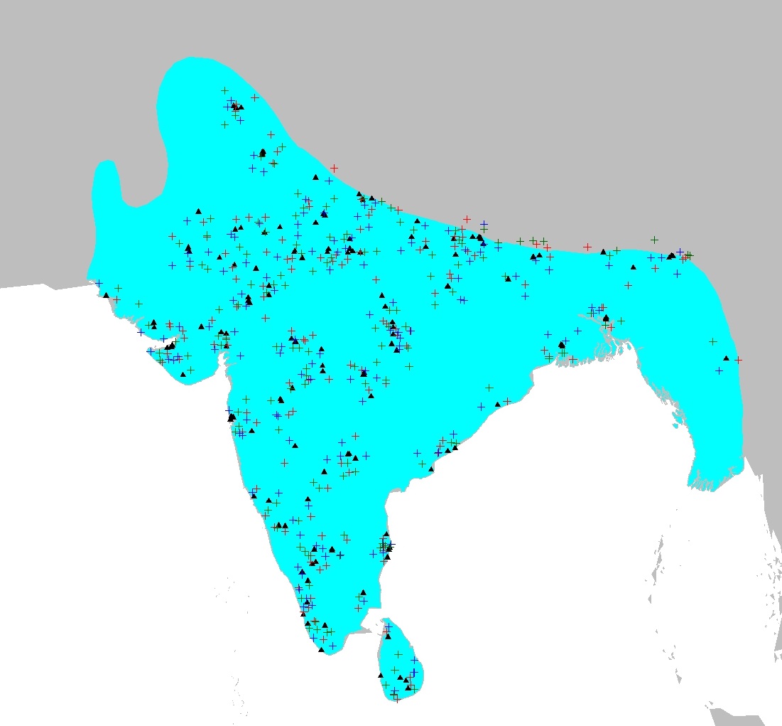
Figure 2.4: Original species occurrences (in black) and the three replicates generated according to coordinates uncertainty (in red, green and blue)

In the picture above (Figure 2.4), triangles represent original species occurrences and coloured cross indicate replicated points. We create the new dataset, including 3 replicates of 197 occurrences each:

> krameri<-resampling

This is finally the definite dataset that we will use to train the SDM.Save it!

> save(krameri, file="krameri.training")