Species Distribution Modelling (SDM): A Guide

Section outline

• Select section Species Distribution Modelling (SDM)

  Species Distribution Modelling (SDM)

  Collapse all Expand all

  
  
• Select section Introduction

  Introduction

  • Select activity About this Tutorial

    

    About this Tutorial Book

    A brief description of rationale, aim and structure of the tutorial.
  • Select activity Tutorial R

    

    Tutorial R File

    Text file with "R" tutorial for the modules.
  • Select activity Scripts and procedures

    

    Scripts and procedures File

    Script and procedures to be used for this tutorial.
  • Select activity Shape file for the P. Kramer

    

    Shape file for the P. Kramer

    Shape file for the P. krameri (species used in this tutorial). 
  • Select activity maxent

    

    maxent File
• Select section Module I – Occurrence data

  Module I – Occurrence data

  In this first module we will see where to find occurrence data (if you don’t have your own), how to download them. Furthermore we will focus of cleaning and validation procedures in order to have a suitable dataset to be use in module 2.

  • Select activity Occurence data

    

    Occurence data Book
• Select section Module II - The environmental variables

  Module II - The environmental variables

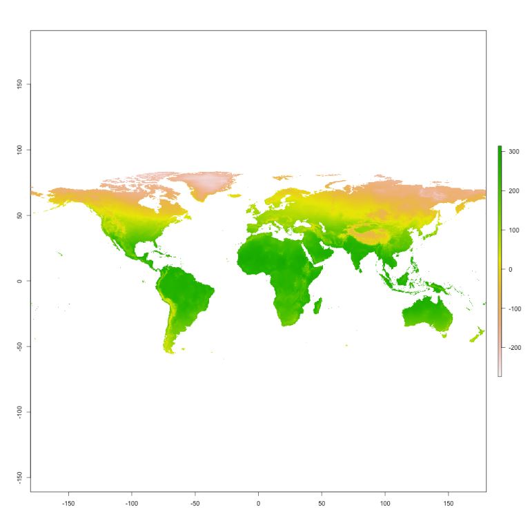
  In this module we will see where and how find environmental layers to build our SDM. Then we will refine again our dataset taking into account the spatial resolution of the environmental layer. Finally, we will see how to deal with the problem of multi-collinearity in environmental layers. At the end on this module we will have a dataset with occurrences and a number of layer that we will use to train our SDM in module 3. 

  • Select activity The environmental variables

    

    The environmental variables Book
• Select section Module III – Running the analysis

  Module III – Running the analysis

  In this module we will use the dataset obtained in module 2 to train the SDMs (occurrences + bioclimatic variables). We produce an SDM for P. krameri under the current climatic conditions and then we will project the model’s results in space (at global level) and in time taking into account the current and the future ("worst" IPCC Fifth Report scenario for the 2070, see also IPCC, 2013) climate conditions. The final training of the model will be performed using an ensemble forecasting approach based on the use of multiple modelling algorithms and the average of the respective predictions (see Thuiller et al., 2009).

  • Select activity Running the analysis

    

    Running the analysis Book
• Select section Module IV - The output interpretation and test of robustness

  Module IV - The output interpretation and test of robustness

  In this module we will build the final model by averaging the 3 ensemble models (one for each replicate) obtained in module 3. A weighted average will be obtained by using the TSS scores associated to each ensemble model that will be extracted and plotted with the ROC scores as well.

  • Select activity The output interpretation and test of robustness

    

    The output interpretation and test of robustness Book
• Select section Module V - A survey of available software

  Module V - A survey of available software

  Not only R is available to realize SDMs. Here we provide a survey of some of the most common used packages for SDM

  • R packages: Dismo, biomod2, maxlike, hSDM, SDMTools
  • Maxent
  • Openmodeller
  • ModEco: Integrated Software for Species Distribution Analysis and Modeling
• Select section Comments and Feedback

  Comments and Feedback

  • Select activity Post here your comments...

    

    Post here your comments... Forum