The environmental variables
| Site: | LifeWatch ERIC Training Platform |
| Course: | Species Distribution Modelling (SDM): A Guide |
| Book: | The environmental variables |
| Printed by: | Guest user |
| Date: | Tuesday, 15 September 2026, 1:48 PM |
Description
In this module we will see where and how find environmental layers to build our SDM. Then we will refine again our dataset taking into account the spatial resolution of the environmental layer. Finally, we will see how to deal with the problem of multi-collinearity in environmental layers. At the end on this module we will have a dataset with occurrences and a number of layer that we will use to train our SDM in module 3.
Table of contents
- 1. Overview
- 2. Where to find environmental variables?
- 3. Choose and download the environmental layers.
- 4. Remove duplicates within the same raster cell
- 5. Reducing the sampling bias with subsampling procedures
- 6. Coordinates uncertainty: how to deal with this issue
- 7. Preparing the model training area
- 8. Dealing with multi-collinearity: Pearson’s R and variance inflation factor analysis
- 9. References
Overview
In this module we will show where and how find environmental layers to build our SDM. Then, we will refine again our dataset taking into account the spatial resolution of the environmental layer. Finally, the problem of multi-collinearity in environmental layers. At the end on this module we will have a dataset with occurrences and a number of layer that we will use to train our SDM in module 3
Where to find environmental variables?
Together with presence data, that will represent the dependant variable in our SDM, we need an independent variable: the predictors.
In SDM we need to add information from spatially referenced data layers to predicting the probability of occurrence of a species throughout the area of interest.
The quality and relevance of the environmental data is crucial.
It is one of the main factor (but not the only) that determines the quality of SDM output maps.
We need environmental layer with a resolution that can provide a good extrapolation of habitat suitability according to the scale of interest
(regional, continental, global), but that not compromise the analysis in term of
computational time and that take into account the uncertainty of the
occurrences.
The right chose is thus a compromise between statistical robustness, user experience and practical aspects.
The environmental layer used must represent the habitat requirements. Many sources on the web provide free environmental raster layers
such as temperature, precipitation, elevation, soil type, land use, etc.
We can use remote sensed data from MODIS (http://modis.gsfc.nasa.gov) or COPERNICUS (http://www.copernicus.eu), or interpolated climatic raster (i.e. the Worldclima
database, www.worldclim.org) or soil database (i.e.the European Soil Portal,
http://eusoils.jrc.ec.europa.eu/).
The choice of the layer to use is driven by the variables the best describe habitat requirements of the species of interest.
However, if you want project your models in the past and in the future, usually interpolated climatic data are often the only source environmental available.
However, also if in some cases climatic data only cannot be consider as the best choice, they usually represent a good because plant and animal species respond very well to climatic changes over hundred or thousand of years.
Climatic data can give good results also for species that are apparently not directly influenced by climate, as subterranean mammals (see Feuda et al., in press).
Choose and download the environmental layers.
In this tutorial we will use environmental layers from the Worldclim database ( www.worldclim.org) that provides climatic data for current condition at different spatial resolution (approximately 1, 4 and 10 square Km). Worldclim environmental layers comprise 19 bioclimatic variables.
We choose to use the resolution at 2.5 arc-minutes (approximately 5 square Km) because is a good compromise between computational efforts and resolution.
First of all we need to download the raster layers. You can do this directly from the website or, better, using an R functions in the library “raster” to download and manipulate layers (the total download data are 123.3 Mb, it will take a while depending of your connection speed):
> library(raster)
> r <- getData("worldclim", var="bio", res=2.5)
l'URL 'http://biogeo.ucdavis.edu/data/climate/worldclim/1_4/grid/cur/bio_2-5m_bil.zip' Content type 'application/zip' length 129319755 bytes (123.3 Mb)
URL aperto
==================================================
downloaded 123.3 Mb
rgdal: version: 0.8-16, (SVN revision 498)
Geospatial Data Abstraction Library extensions to R successfully loaded
Loaded GDAL runtime: GDAL 1.11.0, released 2014/04/16
Path to GDAL shared files:/Library/Frameworks/R.framework/Versions/3.1/Resources/library/rgdal/gdal
Loaded PROJ.4 runtime: Rel. 4.8.0, 6 March 2012, [PJ_VERSION: 480]
Path to PROJ.4 shared files: /Library/Frameworks/R.framework/Versions/3.1/Resources/library/rgdal/proj
Now we created and r object including all the 19 bioclimatic variables. To get information on resolution, projection, etc. just type r:
> r
class : RasterStack
dimensions : 3600, 8640, 31104000, 19 (nrow, ncol, ncell, nlayers)
resolution : 0.04166667, 0.04166667 (x, y)
extent : -180, 180, -60, 90 (xmin, xmax, ymin, ymax)
coord. ref. : +proj=longlat +datum=WGS84 +ellps=WGS84 +towgs84=0,0,0
names : bio1, bio2, bio3, bio4, bio5, bio6, bio7, bio8, bio9, bio10, bio11, bio12, bio13, bio14, bio15, ...
min values : -278, 9, 8, 64, -86, -559, 53, -278, -501, -127, -506, 0, 0, 0, 0, ...
max values : 319, 213, 96, 22704, 489, 258, 725, 376, 365, 382, 289, 10577, 2437, 697, 265, ...
Now try to plot the first layer bio1 (average annual temperature):
> plot(r$bio1)
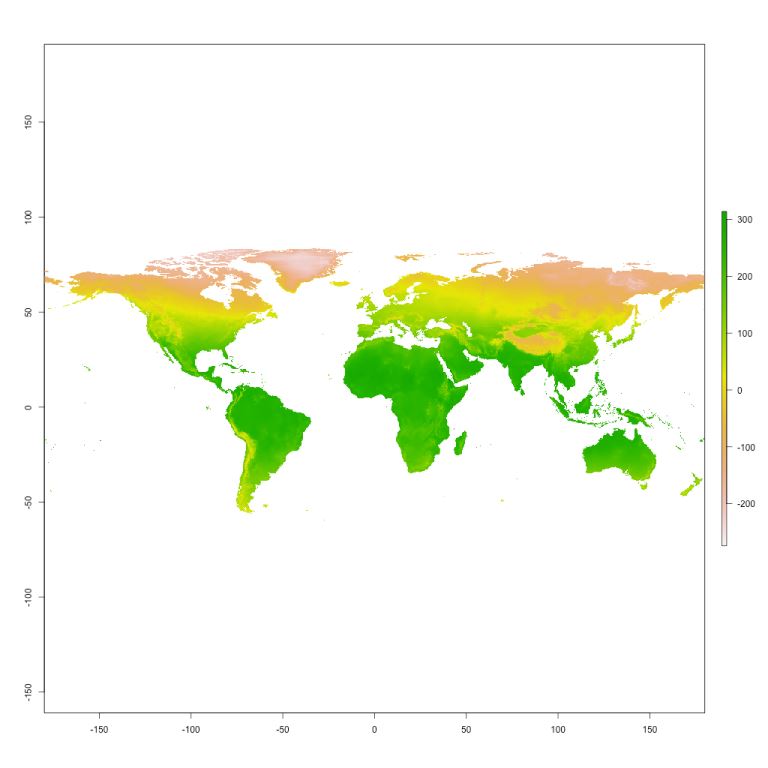
Figure 2.1: Average annual temperature (bio1) downloaded from Worldclim
Our environmental layer (Figure 2.1) was downloaded properly. We can move to the next step
Remove duplicates within the same raster cell
We downloaded layers at a spatial resolution of
approximately 5x5 Km. This means that it is possible that within the same cell
fall more than one occurrence. Despite the coordinates of two occurrences
falling in the same cell can be different, technically they are just a duplicate
of the environmental information provided by the raster. We want to remove this
duplicate (analogously to what we did in Module 1) to remove the potential bias
introduced by duplications. To do this we will use an ad.hoc function written
for this purpose:
occ.desaggregation_RASTER<-function(df, colxy, colvar, rast, plot=T)
{
require(raster)
df_ini<-df
var1<-cellFromXY(rast, df[,colxy])
if(any(is.na(var1))){stop("no NA admitted in species occurrences!")}
var2<-split(var1, var1)
l<-sapply(var2, length)
l1<-l[l>1]
for(j in 1:length(l1))
{
w<-which(var1%in%as.numeric(names(l1[j])))
found<-df[w,]
s<-sample(w,1)
df[w[w!=s],colxy]<-NA
}
df_final<-df[!is.na(df[,colxy[1]]),]
if(plot==T)
{
x11()
plot(df_ini[,colxy],main="distribution of occurences",sub=paste("# initial (black):",nrow(df_ini)," | # kept (red): ",nrow(df_final)),pch=19,col="black",cex=0.5)
points(df_final[,colxy],pch=19,col="red",cex=0.2)
}
return(df_final)
}
Now we apply the new function occ.desaggregation_RASTER to the krameri datasets:
> krameri<-occ.desaggregation_RASTER(df=krameri,colxy=c(2,1), rast=r[[1]], plot=F)
and check the new datafile:
>dim( krameri)
[1] 481
Do you remember the initial number of occurrences downloaded from GBIF? More than 8000. Now we have “only” 481 occurrences!
Reducing the sampling bias with subsampling procedures
Now, since the spatial bias generally results in environmental bias, we have to take account of the last aspect that might introduce the heterogeneous distribution of our occurrence data Plot the last dataset with 481 occurrences:
> library(maptools)
> data(wrld_simpl)
> plot(wrld_simpl)
> points(krameri$lon,krameri$lat, pch=21, bg="red",cex=0.5)
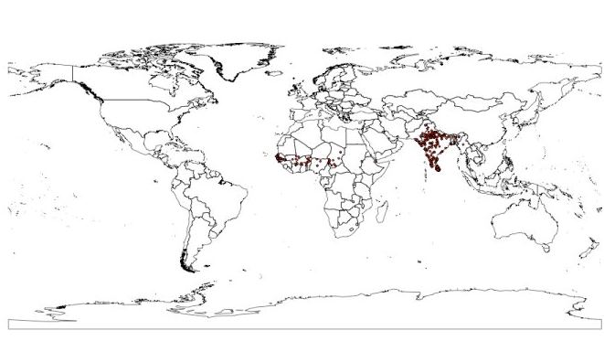
2.2: Occurrences of P. krameri
As you can notice in figure 2, most of the occurrences are concentrated in the Indian sub-continent while less points are in the African sub-Saharan belt. A frequent issue in SDM is an unbalanced spatial distribution of occurrence records, with some areas consistently more sampled than others. If we use this dataset, the environmental information extracted from India occurrences will have a higher weight in the analysis, not because India is more suitable that sub-Saharan area but just because we have more occurrences in that area. A way to deal with this problem is to subsample the occurrences (preferably from the most densely sampled areas) in order to balance the spatial pattern as much as possible. We wrote another ad-hoc function (for further details on the provided function, see Feuda et al., in press).
> source("script/spatial.bias.reduction.R")
> reduction<-spatial.bias.reduction(points=krameri,
xy.cols=c(2,1),
grid.cell.size=50,
mask_base=r[[1]],
FUN="median",
sel.by.err=F,
rep_bsp=1)
P. krameri native range:
>krameri_EOO<-readShapePoly("Shapefile_Pkrameri/Psittacula_krameri_1529_BL.shp")
> krameri_EOO<-krameri_EOO[krameri_EOO@data$ORIGIN==1,]
> plot(krameri_EOO)
> plot(wrld_simpl, add=T)
> plot(krameri_EOO, add=T, col="cyan")
Plot grid used for the subsampling procedure:
> plot(reduction[[2]], add=T)
Plot occurrences pre (blue) and post (red) subsampling procedure (Figure 2.3):
> points(krameri[c(2,1)], pch=19, col="blue",cex=0.5)
> points(reduction[[1]][c(2,1)], pch=19, col="red",cex=0.5)
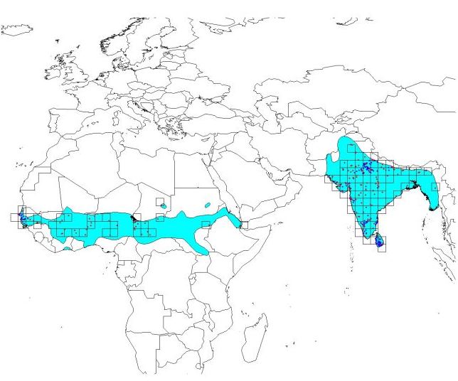
Figure 2.3: Occurrences after the subsamplig procedure. In red the occurrences that will be retained. In blue the occurrences that will be discarded. Cell size
Create the new P. krameri dataset with the subsampled occurrences:
> krameri<-reduction[[1]]
Check the dimension of the new dataset:
> dim(krameri)
[1] 197
After the cleaning, validation and subsampling procedure of Module 1 and 2, our original dataset was reduced to 197 occurrences (we started with more than 8000).
Coordinates uncertainty: how to deal with this issue
A way to obtain a more accurate SDM is to take into account the spatial uncertainty associated to each occurrence. This is particularly relevant when the uncertainty is greater than the spatial resolution of the environmental variables used for training of the model (in our case approximately 5x5 Km). GBIF database provides a specific column reporting the spatial uncertainty in meters.
In this tutorial we will show a function to handle the uncertainty based on a resampling procedure: around each point of presence, a circular buffer with a radius corresponding to the location error is considered. Subsequently, a random point inside each buffer will be generated. The procedure is repeated X times, obtaining X datasets from the first one. Each replicated dataset will be used to train the SDM and the results will be averaged in order to provide a potential species distribution which took into account the spatial uncertainty associated to the coordinates (for further details on this procedure, see Maiorano et al., 2011).
In cases when the coordinates uncertainty is not provided for all records, a way to proceed could be to consider just records with an available uncertainty. If this approach should lead to a too drastic reduction in the number of occurrences, another solution could be to choose a maximum error, according to the scale of your investigation, to be considered for those records without a provided spatial uncertainty.
In the next step we will show how to handle uncertainty for the P. krameri dataset. First of all check in the coordinate uncertainty is provided for all the records:
> summary(krameri$coordUncertaintyM)
| Min. | 1st Qu. | Median | Mean | 3rd Qu. | Max. | NA's |
| 0 | 1 | 1000 | 1709 | 3446 | 4096 | 192 |
We have a good news and a bad one: the uncertainty, when reported, range from 0 to 4096 meters. That's very good for our spatial resolution (approximately 5x5 Km). The bad news is that over 197 records only for 5 of these the coordinates uncertainty was reported. For the remaining 192 records this information is missing. Because we are unable to evaluate the uncertainty and because we are investigating the habitat suitability at a scale that goes from continental to global, we decided to set the uncertainty of the records missing this information to 100 Km (expressed in meters):
> krameri[is.na(krameri[,3]),3]<-100000
and then we proceed with the resampling procedure (function provided)
> source("script/coordinates.precision.resampling.R")
> resampling <- coordinates.precision.resampling(species = krameri, xy.cols = c(2, 1), err = 2500, err.col = 3, vars = r[[1]], rep_cp = 3)
Considering that the resolution of the environmental variables will be 2.5 arc-minutes (≈5 km), the resampling procedure will be applied just to coordinates with a location error greater than 2500 m (“err” argument) (the maximum radius of a buffer completely contained by a raster cell)
> plot(krameri_EOO, col="cyan")
> plot(wrld_simpl, add=T, border="grey", col="grey")
> plot(krameri_EOO, col="cyan", add=T, border="grey")
> plot(SpatialPoints(krameri[c(2,1)]), pch=17, add=T,cex=0.5)
> plot(SpatialPoints(resampling[[1]]), add=T, col="red")
> plot(SpatialPoints(resampling[[2]]),add=T, col="blue")
> plot(SpatialPoints(resampling[[3]]),add=T, col="darkgreen")
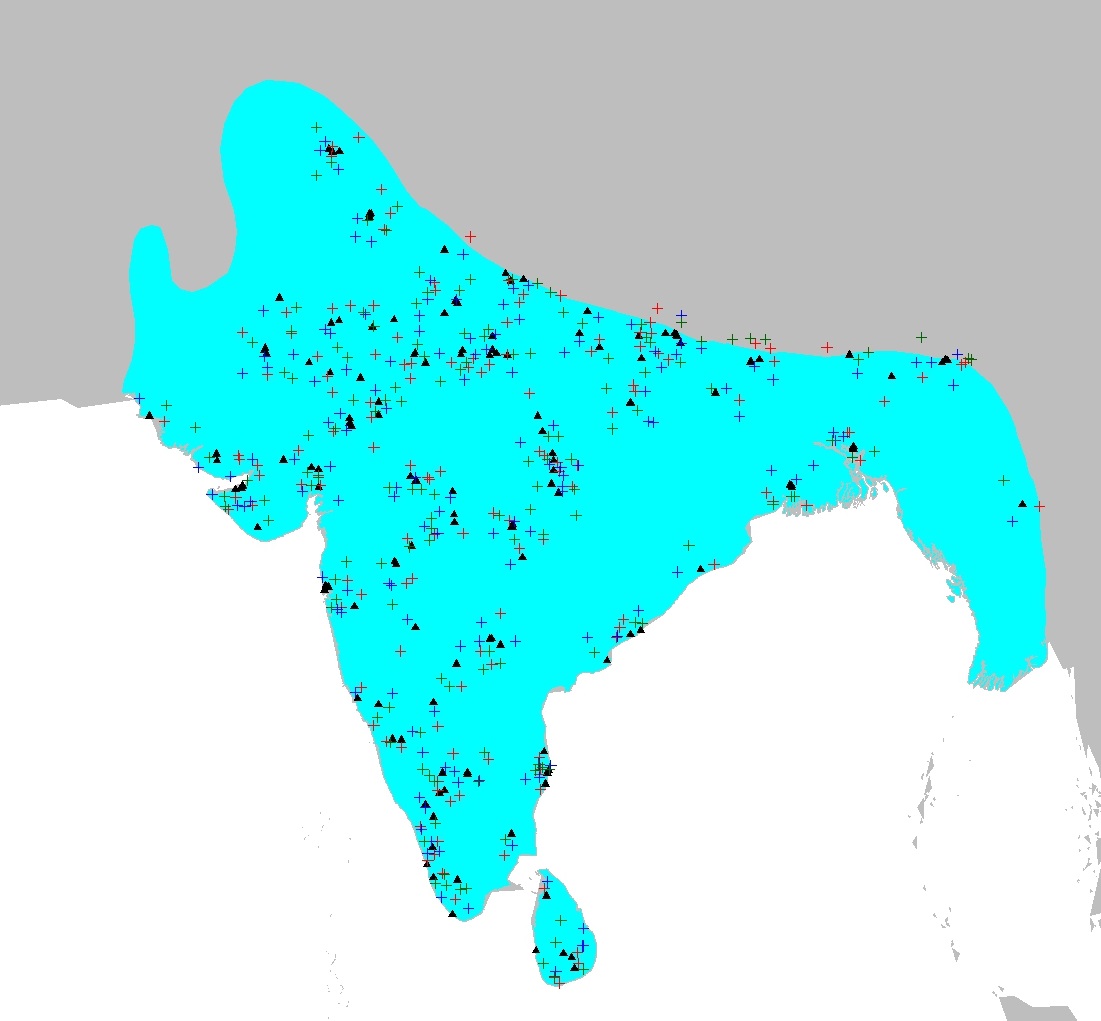
Figure 2.4: Original species occurrences (in black) and the three replicates generated according to coordinates uncertainty (in red, green and blue)
In the picture above (Figure 2.4), triangles represent original species occurrences and coloured cross indicate replicated points. We create the new dataset, including 3 replicates of 197 occurrences each:
> krameri<-resampling
This is finally the definite dataset that we will use to train the SDM.Save it!
> save(krameri, file="krameri.training")
Preparing the model training area
Because P. krameri was not originally distributed worldwide, and we want to create a SDM that take into account the native range of the species, we are going to crop the bioclimatic rasters to create the area used to train the model.
First we will create a buffer around our occurrences points:
>library(rgeos)
>buff<-gBuffer(SpatialPoints(do.call(rbind, krameri)), width=res(r)[1]*100)
The resolution of bioclimatic layers (r) is almost 5 km --> 5km*100=500km
Then, we crop the original layers to the training area delimited by the buffer
>vars<-crop(r, buff, progress="text")
>vars<-mask(vars, buff, progress="text")
Finally we plot the results:
>plot(vars[[1]])
>plot(wrld_simpl, add = T, border = "grey", col = "grey")
>plot(vars[[1]], add=T)
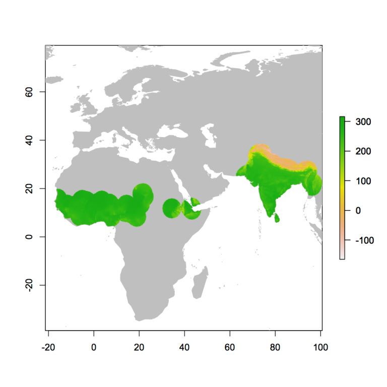
Figure 2.5: Training area
Figure 2.5 shows the bioclimatic variable bio1 (average annual temperature) cropped to the area that we want to use for the training of the model. The same cropping procedure was applied to the other bioclimatic variables.
Dealing with multi-collinearity: Pearson’s R and variance inflation factor analysis
A final step concerns only the environmental variables. The choice of the environmental variables to be included as predictors is a very crucial task. The choice should be take into account the ecological requirements of the species under study but it is important to avoid high degrees of collinearity between the selected predictors. Among the main issues related to collinearity there are: inflation of standard errors on estimates, impossibility to separate variables effects and severe errors in extrapolations in space and time (for further details see Dorman et al., 2013). In this section of the tutorial we provide two so-called “threshold-based” methods that remove predictors correlated over a given threshold: Pearson’s r and the variance inflation factor (VIF) (for details, see Dorman et al., 2013 and Zuur et al., 2010 respectively). Pearson’s r is the most common metric used to evaluate the correlation degree between two numerical predictors. VIF is equal to 1 / (1 - R squared), which reflects the degree to which the variance of an estimated regression coefficient (in a model using these variables as predictors) is increased due only to the correlations among covariates.
First we extract values of environmental rasters in 10000 random points within our training area:
sample<-randomPoints(vars, 10000)
vars_tab<-extract(vars, sample)
Then we calculate the Pearson's r and check which variables have a Pearson's r greater than 0.7:
> abs(cor(vars_tab))>0.7
| bio1 | bio2 | bio3 | bio4 | bio5 | bio6 | bio7 | bio8 | bio9 | bio10 | bio11 | bio12 | bio13 | bio14 | bio15 | bio16 | bio17 | bio18 | bio19 | |
| bio1 | TRUE | FALSE | FALSE | FALSE | FALSE | FALSE | FALSE | FALSE | TRUE | TRUE | TRUE | FALSE | FALSE | FALSE | FALSE | FALSE | FALSE | FALSE | FALSE |
| bio2 | FALSE | TRUE | FALSE | FALSE | TRUE | FALSE | TRUE | FALSE | FALSE | FALSE | FALSE | FALSE | FALSE | FALSE | FALSE | FALSE | FALSE | FALSE | FALSE |
| bio3 | FALSE | FALSE | TRUE | TRUE | FALSE | TRUE | TRUE | FALSE | FALSE | FALSE | TRUE | FALSE | FALSE | FALSE | FALSE | FALSE | FALSE | FALSE | FALSE |
| bio4 | FALSE | FALSE | TRUE | TRUE | FALSE | TRUE | TRUE | FALSE | FALSE | FALSE | TRUE | FALSE | FALSE | FALSE | FALSE | FALSE | FALSE | FALSE | FALSE |
| bio5 | FALSE | TRUE | FALSE | FALSE | TRUE | FALSE | FALSE | FALSE | FALSE | TRUE | FALSE | FALSE | FALSE | FALSE | FALSE | FALSE | FALSE | FALSE | FALSE |
| bio6 | FALSE | FALSE | TRUE | TRUE | FALSE | TRUE | TRUE | FALSE | FALSE | FALSE | TRUE | FALSE | FALSE | FALSE | FALSE | FALSE | FALSE | FALSE | FALSE |
| bio7 | FALSE | TRUE | TRUE | TRUE | FALSE | TRUE | TRUE | FALSE | FALSE | FALSE | FALSE | FALSE | FALSE | FALSE | FALSE | FALSE | FALSE | FALSE | FALSE |
| bio8 | FALSE | FALSE | FALSE | FALSE | FALSE | FALSE | FALSE | TRUE | FALSE | TRUE | FALSE | FALSE | FALSE | FALSE | FALSE | FALSE | FALSE | FALSE | FALSE |
| bio9 | TRUE | FALSE | FALSE | FALSE | FALSE | FALSE | FALSE | FALSE | TRUE | FALSE | TRUE | FALSE | FALSE | FALSE | FALSE | FALSE | FALSE | FALSE | FALSE |
| bio10 | TRUE | FALSE | FALSE | FALSE | TRUE | FALSE | FALSE | TRUE | FALSE | TRUE | FALSE | FALSE | FALSE | FALSE | FALSE | FALSE | FALSE | FALSE | FALSE |
| bio11 | TRUE | FALSE | TRUE | TRUE | FALSE | TRUE | FALSE | FALSE | TRUE | FALSE | TRUE | FALSE | FALSE | FALSE | FALSE | FALSE | FALSE | FALSE | FALSE |
| bio12 | FALSE | FALSE | FALSE | FALSE | FALSE | FALSE | FALSE | FALSE | FALSE | FALSE | FALSE | TRUE | TRUE | FALSE | FALSE | TRUE | FALSE | TRUE | FALSE |
| bio13 | FALSE | FALSE | FALSE | FALSE | FALSE | FALSE | FALSE | FALSE | FALSE | FALSE | FALSE | TRUE | TRUE | FALSE | FALSE | TRUE | FALSE | FALSE | FALSE |
| bio14 | FALSE | FALSE | FALSE | FALSE | FALSE | FALSE | FALSE | FALSE | FALSE | FALSE | FALSE | FALSE | FALSE | TRUE | FALSE | FALSE | TRUE | FALSE | FALSE |
| bio15 | FALSE | FALSE | FALSE | FALSE | FALSE | FALSE | FALSE | FALSE | FALSE | FALSE | FALSE | FALSE | FALSE | FALSE | TRUE | FALSE | FALSE | FALSE | FALSE |
| bio16 | FALSE | FALSE | FALSE | FALSE | FALSE | FALSE | FALSE | FALSE | FALSE | FALSE | FALSE | TRUE | TRUE | FALSE | FALSE | TRUE | FALSE | FALSE | FALSE |
| bio17 | FALSE | FALSE | FALSE | FALSE | FALSE | FALSE | FALSE | FALSE | FALSE | FALSE | FALSE | FALSE | FALSE | TRUE | FALSE | FALSE | TRUE | FALSE | FALSE |
| bio18 | FALSE | FALSE | FALSE | FALSE | FALSE | FALSE | FALSE | FALSE | FALSE | FALSE | FALSE | TRUE | FALSE | FALSE | FALSE | FALSE | FALSE | TRUE | FALSE |
| bio19 | FALSE | FALSE | FALSE | FALSE | FALSE | FALSE | FALSE | FALSE | FALSE | FALSE | FALSE | FALSE | FALSE | FALSE | FALSE | FALSE | FALSE | FALSE | TRUE |
From this output we can understand that bio1 is highly correlated with bio5, bio6, bio8, bio9, bio10 and bio11. Other bioclimatic variables show high levels of correlation. Now we need to select predictors (with r>0.7) to be removed. This choice is somehow arbitrary. For instance in the case of bio1-bio10 we can remove bio1 or bio10. Usually one will choose to retain those variables that have a “biological meaning” for the specie of interest, on the basis of your experience. We will choose to retain 7 variables:
>abs(cor(vars_tab[-c(3,4,5,6,8,9,10,11,13,14,16,18), -c(3,4,5,6,8,9,10,11,13,14,16,18)])) > 0.7
| bio1 | bio2 | bio7 | bio12 | bio15 | bio17 | bio19 | |
| bio1 | TRUE | FALSE | FALSE | FALSE | FALSE | FALSE | FALSE |
| bio2 | FALSE | TRUE | FALSE | FALSE | FALSE | FALSE | FALSE |
| bio7 | FALSE | FALSE | TRUE | FALSE | FALSE | FALSE | FALSE |
| bio12 | FALSE | FALSE | FALSE | TRUE | FALSE | FALSE | FALSE |
| bio15 | FALSE | FALSE | FALSE | FALSE | TRUE | FALSE | FALSE |
| bio17 | FALSE | FALSE | FALSE | FALSE | FALSE | TRUE | FALSE |
| bio19 | FALSE | FALSE | FALSE | FALSE | FALSE | FALSE | TRUE |
According to Pearson's R we create the new set of rasters including only the bioclimatic variables chosen:
> vars_r <- vars[[-c(3,4,5,6,8,9,10,11,13,14,16,18)]]
Now we try with VIF test, the variance inflation factor analysis (function provided with the tutorial)
> source("script/vif_functions.R")
this function find and remove each predictor reporting a VIF greater than 3
> vars_vif<-vif(vars, thresh=3, trace=F)
We create a new set of rasters according with VIF:
> vars_vif<-r[[which(names(r)%in%vars_vif)]]
and finally we compare raster dataset based respectively on Pearson,s r and VIF:
> names(vars_r)
[1] "bio1" "bio2" "bio7" "bio12" "bio15" "bio17" "bio19"
> names(vars_vif)
[1] "bio2" "bio3" "bio8" "bio13" "bio14" "bio15" "bio18" "bio19"
The two procedures show some differences in the number and type of raster layers selected. Pearson's r seems to be more conservative than the VIF. Furthermore, Pearson's r allow a certain degree of arbitrariness respect to VIF (where you have to choose a threshold value) because the researcher must operate a choice of the variables to retain. To train model in the module 3 we decided to use layeres selected on the basis of the Pearson correlation test. We create a new directory where we will store the selected variables
> dir.create("predictors")
> writeRaster(vars_r, "predictors/", bylayer=T, suffix="names")
References
Feuda R, Bannikova AA, Zemlemerova ED, Di Febbraro M, Loy A, Hutterer R, Aloise G, Zykov A, Annesi F, Colangelo P. 2015. Tracing the evolutionary history of Talpa europaea through mtDNA phylogeography and species distribution modelling. Biological Journal of the Linnean Society, in press.
Dormann CF, Elith J, Bacher S, Buchmann C, Carl G, Carré G, Garcìa Marquéz JR, Gruber B, Lafourcade B, Leitão PJ, Münkemüller T, McClean C, Osborne PE, Reineking B, Schröder B, Skidmore AK, Zurell D, Lautenbach S. 2013. Collinearity: a review of methods to deal with it and a simulation study evaluating their performance. Ecography 36: 27–46.
Maiorano L, Falcucci A, Zimmermann NE, Psomas A, Pottier J, Baisero D, Rondinini C, Guisan A, Boitani L. 2011. The future of terrestrial mammals in the Mediterranean basin under climate change. Phil. Trans. R. Soc. B, 366, 2681–2692.
Zuur AF, Ieno EN, Elphick CS. 2010. A protocol for data exploration to avoid common statistical problems. Methods in Ecology & Evolution 2010, 1, 3–14