The environmental variables
In this module we will see where and how find environmental layers to build our SDM. Then we will refine again our dataset taking into account the spatial resolution of the environmental layer. Finally, we will see how to deal with the problem of multi-collinearity in environmental layers. At the end on this module we will have a dataset with occurrences and a number of layer that we will use to train our SDM in module 3.
Reducing the sampling bias with subsampling procedures
Now, since the spatial bias generally results in environmental bias, we have to take account of the last aspect that might introduce the heterogeneous distribution of our occurrence data Plot the last dataset with 481 occurrences:
> library(maptools)
> data(wrld_simpl)
> plot(wrld_simpl)
> points(krameri$lon,krameri$lat, pch=21, bg="red",cex=0.5)
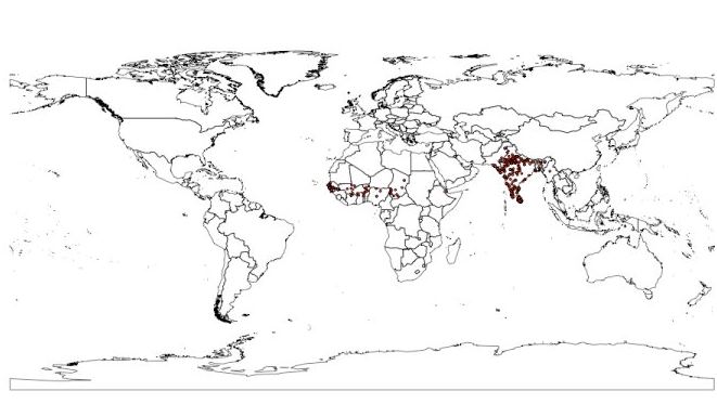
2.2: Occurrences of P. krameri
As you can notice in figure 2, most of the occurrences are concentrated in the Indian sub-continent while less points are in the African sub-Saharan belt. A frequent issue in SDM is an unbalanced spatial distribution of occurrence records, with some areas consistently more sampled than others. If we use this dataset, the environmental information extracted from India occurrences will have a higher weight in the analysis, not because India is more suitable that sub-Saharan area but just because we have more occurrences in that area. A way to deal with this problem is to subsample the occurrences (preferably from the most densely sampled areas) in order to balance the spatial pattern as much as possible. We wrote another ad-hoc function (for further details on the provided function, see Feuda et al., in press).
> source("script/spatial.bias.reduction.R")
> reduction<-spatial.bias.reduction(points=krameri,
xy.cols=c(2,1),
grid.cell.size=50,
mask_base=r[[1]],
FUN="median",
sel.by.err=F,
rep_bsp=1)
P. krameri native range:
>krameri_EOO<-readShapePoly("Shapefile_Pkrameri/Psittacula_krameri_1529_BL.shp")
> krameri_EOO<-krameri_EOO[krameri_EOO@data$ORIGIN==1,]
> plot(krameri_EOO)
> plot(wrld_simpl, add=T)
> plot(krameri_EOO, add=T, col="cyan")
Plot grid used for the subsampling procedure:
> plot(reduction[[2]], add=T)
Plot occurrences pre (blue) and post (red) subsampling procedure (Figure 2.3):
> points(krameri[c(2,1)], pch=19, col="blue",cex=0.5)
> points(reduction[[1]][c(2,1)], pch=19, col="red",cex=0.5)
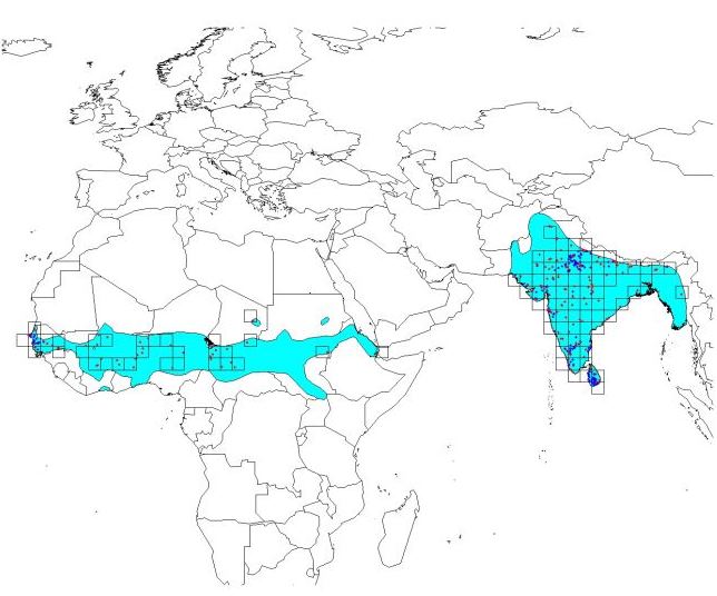
Figure 2.3: Occurrences after the subsamplig procedure. In red the occurrences that will be retained. In blue the occurrences that will be discarded. Cell size
Create the new P. krameri dataset with the subsampled occurrences:
> krameri<-reduction[[1]]
Check the dimension of the new dataset:
> dim(krameri)
[1] 197
After the cleaning, validation and subsampling procedure of Module 1 and 2, our original dataset was reduced to 197 occurrences (we started with more than 8000).