The environmental variables
In this module we will see where and how find environmental layers to build our SDM. Then we will refine again our dataset taking into account the spatial resolution of the environmental layer. Finally, we will see how to deal with the problem of multi-collinearity in environmental layers. At the end on this module we will have a dataset with occurrences and a number of layer that we will use to train our SDM in module 3.
Choose and download the environmental layers.
In this tutorial we will use environmental layers from the Worldclim database ( www.worldclim.org) that provides climatic data for current condition at different spatial resolution (approximately 1, 4 and 10 square Km). Worldclim environmental layers comprise 19 bioclimatic variables.
We choose to use the resolution at 2.5 arc-minutes (approximately 5 square Km) because is a good compromise between computational efforts and resolution.
First of all we need to download the raster layers. You can do this directly from the website or, better, using an R functions in the library “raster” to download and manipulate layers (the total download data are 123.3 Mb, it will take a while depending of your connection speed):
> library(raster)
> r <- getData("worldclim", var="bio", res=2.5)
l'URL 'http://biogeo.ucdavis.edu/data/climate/worldclim/1_4/grid/cur/bio_2-5m_bil.zip' Content type 'application/zip' length 129319755 bytes (123.3 Mb)
URL aperto
==================================================
downloaded 123.3 Mb
rgdal: version: 0.8-16, (SVN revision 498)
Geospatial Data Abstraction Library extensions to R successfully loaded
Loaded GDAL runtime: GDAL 1.11.0, released 2014/04/16
Path to GDAL shared files:/Library/Frameworks/R.framework/Versions/3.1/Resources/library/rgdal/gdal
Loaded PROJ.4 runtime: Rel. 4.8.0, 6 March 2012, [PJ_VERSION: 480]
Path to PROJ.4 shared files: /Library/Frameworks/R.framework/Versions/3.1/Resources/library/rgdal/proj
Now we created and r object including all the 19 bioclimatic variables. To get information on resolution, projection, etc. just type r:
> r
class : RasterStack
dimensions : 3600, 8640, 31104000, 19 (nrow, ncol, ncell, nlayers)
resolution : 0.04166667, 0.04166667 (x, y)
extent : -180, 180, -60, 90 (xmin, xmax, ymin, ymax)
coord. ref. : +proj=longlat +datum=WGS84 +ellps=WGS84 +towgs84=0,0,0
names : bio1, bio2, bio3, bio4, bio5, bio6, bio7, bio8, bio9, bio10, bio11, bio12, bio13, bio14, bio15, ...
min values : -278, 9, 8, 64, -86, -559, 53, -278, -501, -127, -506, 0, 0, 0, 0, ...
max values : 319, 213, 96, 22704, 489, 258, 725, 376, 365, 382, 289, 10577, 2437, 697, 265, ...
Now try to plot the first layer bio1 (average annual temperature):
> plot(r$bio1)
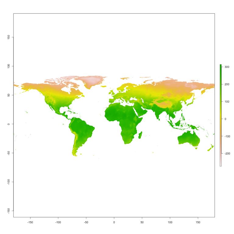
Figure 2.1: Average annual temperature (bio1) downloaded from Worldclim
Our environmental layer (Figure 2.1) was downloaded properly. We can move to the next step