Occurence data
In this first module we will see where to find occurrence data (if you don’t have your own), how to download them. Furthermore we will focus of cleaning and validation procedures in order to have a suitable dataset to be use in module 2.
Visual check and filtering of data with IUCN EOOs Step 2/4
Ok, we have several occurrence data around the world (Fig. 1.1). However, we are interested to model the habitat suitability of this species using occurrences only from its native range (this species has been introduced worldwide by humans). It is possible to download a shapefile with the original range of the species from the IUCN website (http://www.iucnredlist.org/details/22685441/0). Then we can add the native range to our map. First you have to load the shape file (provided with the tutorial):
> krameri_EOO<-readShapePoly("Shapefile_Pkrameri/Psittacula_krameri_1529_BL.shp")
> krameri_EOO<-krameri_EOO[krameri_EOO@data$ORIGIN==1,]
Then we can plot the P. krameri native range on the world map (Fig. 1.2):
> plot(wrld_simpl)
> plot(krameri_EOO, col="cyan", add=T)
> xy<-cbind(krameri$lon, krameri$lat)
> points(xy, pch=21, bg="red",cex=0.5)
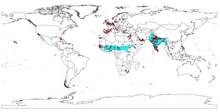
Figure 1.2: The native range of P. krameri (in blue) was superimposed to the map. Most occurences fall outside the native range