Occurence data
| Site: | LifeWatch ERIC Training Platform |
| Course: | Species Distribution Modelling (SDM): A Guide |
| Book: | Occurence data |
| Printed by: | Guest user |
| Date: | Tuesday, 15 September 2026, 2:35 PM |
Description
In this first module we will see where to find occurrence data (if you don’t have your own), how to download them. Furthermore we will focus of cleaning and validation procedures in order to have a suitable dataset to be use in module 2.
Overview
In this first module we will see where to find occurrence data (if you don’t have your own), how to download them. Furthermore we will focus of cleaning and validation procedures in order to have a suitable dataset to be use in module 2.
Where to find occurrence data?
Ideally, the user should have a file, in txt, csv or other suitable formats for R, providing the coordinates of spatial occurrences of the species under study. If the aim of the study is to build the potential distribution of a species over a large area (continental or global scale), it is a common practice to gather spatial data from online databases that have being collecting and freely providing species records in recent years. The Global Biodiversity Information Facility (GBIF; http://www.gbif.org ) provides a huge amount of occurrences data and it is a good source to gather information on spatial distribution of species. There are also many other database, focusing on specific groups, such as HerpNET2 (http://herpnet2.org ), MaNIS (http://manisnet.org), FishNET2 (http://fishnet2.net) and many others.
Importing occurrence data
The package dismo provide a function to direct download occurrence data from GBIF. We will use this function to download the occurrence data of the rose-ringed parakeet (Psittacula krameri)
> library(dismo)
> krameri<-gbif(genus="Psittacula", species="krameri", geo=T, concept=T)
The arguments geo=T tell to the function to download only those records provided with latitude and longitude. The arguments concept=T tells to the function to download also the data from subspecies.
Now we check which kind of information we downloaded:
> colnames(krameri)
| [1] | "species" | "continent" | "country" | "adm1" |
| [5] | "adm2" | "locality" | "lat" | "lon" |
| [9] | "coordUncertaintyM" | "alt" | "institution" | "collection" |
| [13] | "catalogNumber" | "basisOfRecord" | "collector" | "earliestDateCollected" |
| [17] | "latestDateCollected" | "gbifNotes" | "downloadDate" | "maxElevationM" |
| [21] | "minElevationM" | "maxDepthM" | "minDepthM" | "ISO2" |
| [25] | "cloc" |
There are 25 variables. We are interested in latitude (lat), longitude (lon) and uncertainity associated to coordinates (coordUncertaintyM). Just for our convenience we will discard other information:
> krameri<-krameri[,c(7:9)]
Now we have the data, composed by three variables, necessary to start. First of all we want check the composition of the dataset with the R functions head(), summary() and str():
> head(krameri)
| lat | lon | coordUncertaintyM | |
| 1 | -20.083300 | 57.58330 | <NA> |
| 2 | -20.083300 | 57.58330 | <NA> |
| 3 | -20.450000 | 57.66670 | <NA> |
| 4 | -20.083300 | 57.58330 | <NA> |
| 5 | 19.766666 | 85.33336 | <NA> |
| 6 | 9.511201 | 76.35395 | <NA> |
> summary(krameri$lat)
| Min. | 1st Qu. | Median | Mean | 3rd Qu. | Max. | NA's |
| -37.92 | 24.55 | 28.53 | 33.19 | 51.38 | 60.40 | 7 |
> str(krameri)
'data.frame' : 8078 obs. of 3 variables:
$ lat: num -20.1 -20.1 -20.4 -20.1 19.8 ...
$ lon: num 57.6 57.6 57.7 57.6 85.3 ...
$ coordUncertaintyM: chr NA NA NA NA ...
From the inspection of the dataset emerge that there are some missing coordinates (NAs) and that the coordinates uncertainty was loaded as character vector instead that numeric vector. We change "coordUncertaintyM" from character to numeric:
> krameri$coordUncertaintyM <-as.numeric(krameri$coordUncertaintyM)
Clean the dataset
Often datasets downloaded need to be checked for errors that might create some fatal errors in our analysis or produce wrong results. The most common problem are zeros and missing data in the coordinates. Another problem are the duplicated coordinates. So the first step is to clean the dataset We start removing specimens with missing coordinates:
> krameri<-krameri[!is.na(krameri$lat),]
Because duplicated records (i.e. multiple records with identical coordinates) may introduce a bias in the analysis, we exclude the duplicated records and check for the number or record still present:
> xy<-cbind(krameri$lon,krameri$lat)
> dup<-duplicated(xy)
> krameri<-krameri[!dup,]
> dim(krameri)
[1] 2309 3
We started with 8078 records and after the cleaning procedure we have 2039 records.
Visual check and filtering of data with IUCN EOOs
In this section we will see, in four steps, how to visually check our data plotting the occurrences on a map
Visual check and filtering of data with IUCN EOOs Step 1/4
The next step is to visually inspect the dataset plotting the occurrences on a map (Figure 1):
> library(maptools)
> data(wrld_simpl)
> plot(wrld_simpl)
> points(krameri$lon,krameri$lat, pch=21, bg="red",cex=0.5)
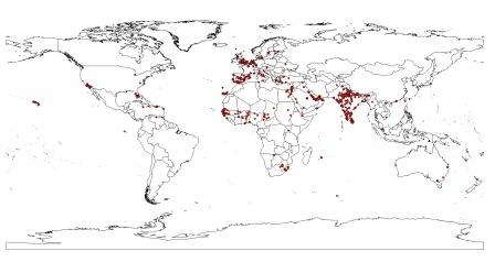
Figure 1.1: A map showing the occurences of P. krameri downloaded from GBIF.
Visual check and filtering of data with IUCN EOOs Step 2/4
Ok, we have several occurrence data around the world (Fig. 1.1). However, we are interested to model the habitat suitability of this species using occurrences only from its native range (this species has been introduced worldwide by humans). It is possible to download a shapefile with the original range of the species from the IUCN website (http://www.iucnredlist.org/details/22685441/0). Then we can add the native range to our map. First you have to load the shape file (provided with the tutorial):
> krameri_EOO<-readShapePoly("Shapefile_Pkrameri/Psittacula_krameri_1529_BL.shp")
> krameri_EOO<-krameri_EOO[krameri_EOO@data$ORIGIN==1,]
Then we can plot the P. krameri native range on the world map (Fig. 1.2):
> plot(wrld_simpl)
> plot(krameri_EOO, col="cyan", add=T)
> xy<-cbind(krameri$lon, krameri$lat)
> points(xy, pch=21, bg="red",cex=0.5)
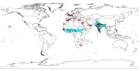
Figure 1.2: The native range of P. krameri (in blue) was superimposed to the map. Most occurences fall outside the native range
Visual check and filtering of data with IUCN EOOs Step 3/4
Many records fall outside the native range. We will refine the dataset removing those records:
> krameri_sp<-SpatialPoints(xy)
> ov<-over(krameri_sp, krameri_EOO)
> krameri<-krameri[!is.na(ov[,1]),]
And we plot again the occurrences on the map:
> plot(wrld_simpl)
> plot(krameri_EOO, col="cyan", add=T)
> xy<-cbind(krameri$lon,krameri$lat)
> points(xy, pch=21, bg="red",cex=0.5)
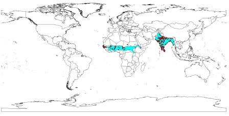
Figure 1.3: The occurences of P. krameri after the removal of occurrences falling outside the native range
Visual check and filtering of data with IUCN EOOs Step 4/4
> dim(krameri)
Now we have a dataset including only records from the native range of the species (n=640).
We save this file ready for module 2:
> write.table(krameri,file="krameri_NativeRange.txt")
In module 2 we will see how to further refine our dataset taking into account the spatial resolution of the environmental layers