Parameter Estimation - Part I
Parameter Estimation (I)
4. Some technicalities
The R instruction mle(LL, start = list(x=0.05, y=0.5), method = "L-BFGS-B", lower = rep(0, 2)) requires a starting point for each variable. Different starting points can give rise to different results, as in Example 10.5.
Example 10.5.
Referring to Example 10.3, two different starting points have been considered:
fit1a <- mle(LL, start = list(x=0.05, y=0.9), method = "L-BFGS-B", lower = rep(0, 2))
summary(fit1a)
Maximum likelihood estimation
Call:
mle(minuslogl = LL, start = list(x = 0.05, y = 0.9), method = "L-BFGS-B", lower = rep(0, 2))
Coefficients:
| Estimate | Std. Error | |
| x | 0.087394825 | 0.033275216 |
| y | 0.001088747 | 0.001620498 |
-2 log L: 126.881
fit1b <- mle(LL, start = list(x=1.5, y=0.1), method = "L-BFGS-B",
+ lower = rep(0, 2))
Error in optim(start, f, method = method, hessian = TRUE, ...) :
L-BFGS-B needs finite values of 'fn'.
Compared to fit1 of Example 10.3, in the case of fit1a, slightly different estimates have been obtained, but the likelihood values are very close. Then, the two estimated models are substantially equivalent.
In the case of fit1b, the command is not able to provide an answer. An error message is displayed referring to the fact that for some values of x and y, the function ("fn", i.e. LL) we are trying to optimize does not have a finite value. This is because in some cases the argument of the logarithm function (see Eq. (10.2)) can be numerically equal to 0, and an “infinite” value obtained. This problem can be solved by choosing different starting values in start.
As in the case of Examples 10.1 and 10.2, it can be useful to look at a plot of the likelihood function to find suitable starting points.
Example 10.6.
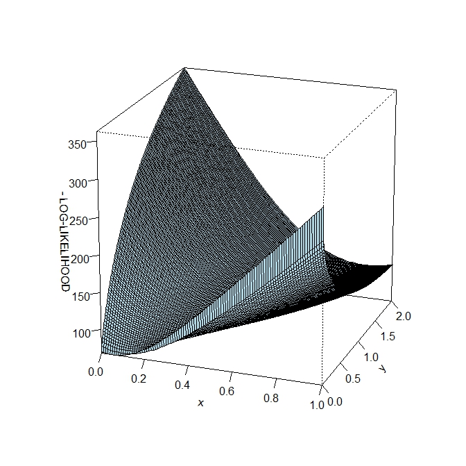
To complete Example 10.3, we provide some instructions to plot the minus-log-likelihood function.
# We define a grid over the domain of the function, that is a set of
# pairs (x,y):
x1<-seq(0,1,by=0.01)
y1<-seq(0,2,by=0.01)
length(x1)
[1] 101
x1[1:10]
[1] 0.00 0.01 0.02 0.03 0.04 0.05 0.06 0.07 0.08 0.09
# and then for each point (x1[k], y1[j]) of the grid we compute the
# value of –LL : these values are stored in a matrix, z
z <- matrix(0,nrow=length(x1), ncol=length(y1))
for(k in 1:length(x1)) {
for(j in 1:length(y1)) { z[k,j]<-LL(x1[k],y1[j]) }
}
persp(x1,y1,-z,phi=20,theta=20,d=10,col="light blue",ticktype="detailed",xlab="x",ylab="y", zlab="- LOG-LIKELIHOOD")
# a useful indication for setting the starting points for the search
# algorithm is the contour plot:
contour(x1,y1,z,col="blue",xlab="x",ylab="y",main="CONTOUR PLOT")
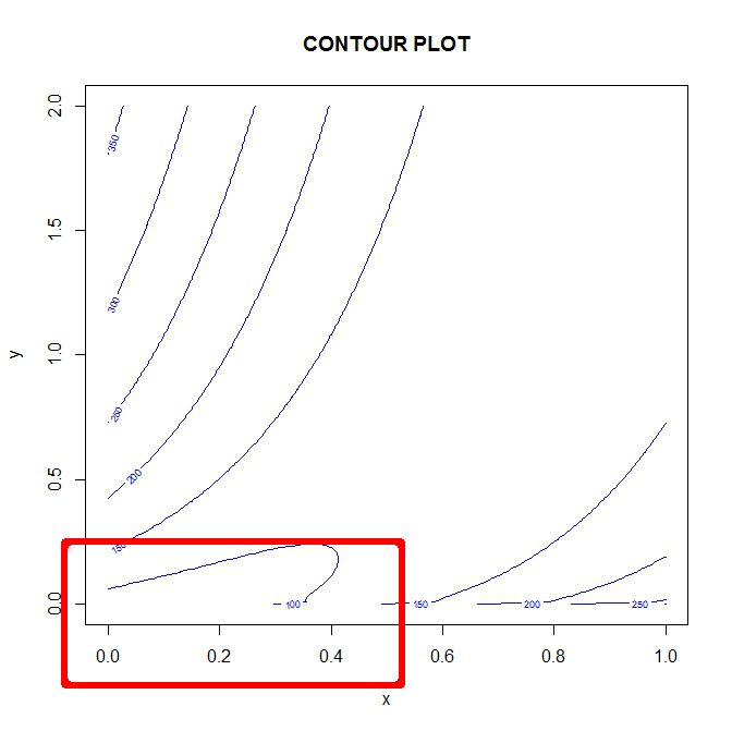
Each line in the contour plot is a level-curve, that is a curve joining all the points (x,y) having the same “z”. As we are searching for a minimum value, the region of interest is the one defined by the lowest level, here 100. Therefore, a suitable choice as start in the mle command is an x value between 0 and about 0.5 and a y value between 0 and about 0.3, or close values.
Summing up, a good practice in this and in many other optimization problems is to run the mle command several times, with different starting points. The highest value of the log-likelihood indicates the best model.