Parameter Estimation - Part I

Site:	LifeWatch ERIC Training Platform
Course:	Spatially explicit metapopulation model - Incidence Function Model
Book:	Parameter Estimation - Part I

Printed by:	Guest user
Date:	Monday, 27 July 2026, 12:18 PM

Description

Parameter Estimation (I)

1. Parameter Estimation (I)
2. Maximum likelihood estimation(MLE)
3. Basic IFM parameterization
4. Some technicalities

1. Parameter Estimation (I)

In all the previous Units we used as a reference metapopulation presence/absence data obtained by simulations from a IFM at equilibrium with parameters A0 = 0.0004, x = 0.05 and y = 0.005. Here we deal with the problem of estimating the unknown parameters of an IFM on the basis of one or more snapshots of presence/absence data.

As mentioned at the end of Unit 1, we will assume that the species behaves as a metapopulation in the fragmented area where it has been observed, and that an IFM is suitable to model the metapopulation dynamics. Then, we will not discuss how to check whether a metapopulation approach is suitable or not.

In particular, we limit ourselves to the case of the basic IFM, with and without the rescue effect and we will not discuss parameter estimation for the time-dependent model. For the basic IFM approach, the maximum likelihood estimation method will be used. A slight variation of this method also applies to the time-dependent IFM. However, in this case a lot of technicalities are required, going beyond the aim of this course. Interested people can refer to Moilanen (1999).

2. Maximum likelihood estimation(MLE)

The working principle of this method is that if the observation process gives rise to certain data, then it is reasonable to assume that the unknown, “true” parameters driving the process are those assigning the highest probability to the observed data. We exemplify this concept in the following two simple examples. In particular, Example 10.1 will be fundamental for the rest of the Unit.

Example 10.1. Coin tossing.
To estimate the probability of getting a "Head" when tossing a coin, a coin has been tossed 5 times obtaining head (H), tail (T), T, T, H. Let $\theta$ the unknown success probability (i.e., the probability of getting a H). The probability of the observed sequence of heads and tails is

P(H,T,T,T,H) = $\theta$ (1- $\theta$) (1- $\theta$) (1- $\theta$) $\theta$ = $\theta$² (1- $\theta$)³

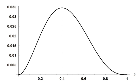
that is, the product of the likelihood of each observation. The following picture shows P(H,T,T,T,H) as a function of $\theta$, i.e. the likelihood function. By the usual derivatives-based techniques it is easy to show that the maximum value of the likelihood is reached for $\theta$ = 2/5= 0.4, the proportion of observed heads.

Example 10.2. Gaussian model.
To estimate the mean tree diameter in a forest, a sample of 10 measures (cm) has been collected:

88.4, 91.5, 83.7, 105.4, 120.5, 97.3, 110.2, 99.5, 80.0, 100.2 .

We assume that the tree diameter follows a Gaussian distribution with unknown mean μ and standard deviation σ.

In analogy with Example 10.1, the likelihood function is the product of the “likelihood” of each collected measure, where the likelihood is given by the Gaussian density:

$$\frac{exp⁡{(-(88.4-μ)^2)⁄(2\sigma^2)}}{\sqrt{(2π\sigma^2)}}×\frac{exp⁡{(-(91.5-μ)^2)⁄(2\sigma^2)}}{\sqrt{(2π\sigma^2)}}×…×\frac{exp⁡{(-(100.2-μ)^2)⁄(2\sigma^2)}}{\sqrt{(2π\sigma^2)}}$$

The two-dimensional likelihood function is shown in the following picture

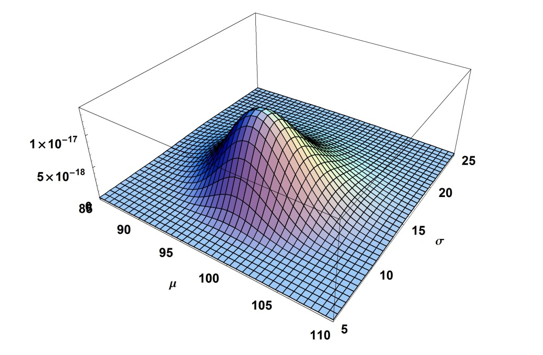
The ML estimates are given by the sample mean 97.67 cm and the sample standard deviation^{^[1]} 11.74 cm.

[1] $n^{-1} \sum_{i=1,…,n}(x_i-\bar{x})^2 $

The main question is to find the likelihood function for the IFM. In the following sections we will answer to this question in the case of only one snapshot of data. The more general case will be considered in Unit 11.

3. Basic IFM parameterization

Let us refer to Example 10.1. The assumptions of the basic model described in Unit 4, possibly modified by Eq. (5.2) to include rescue effect, allows us to consider the n patches as n coins: the main difference is that each patch has his own “success” probability, expressed by the incidence J_i of Eq. (4.1).

For the sake of simplicity, we firstly consider the case of one only snapshot of data. Referring to Example 10.1, this is equivalent to consider 5 coins with five eventually different probabilities θ_i, and only one flip for each coin. This leads to P(H,T,T,T,H) = θ₁ (1- θ₂) (1- θ₃) (1- θ₄) θ₅.

For the IFM, this means that the likelihood function L can be expressed as:

(10.1)$L(x,y│δ_1,…,δ_n )= J_1^{δ_1}(1-J_1)^{1-δ_1}×… × J_n^{δ_n}(1-J_n)^{1-δ_n} $

where the usual Bernoulli notation θ^u (1- θ)^1-u = θ if u = 1 and θ^u (1- θ)^1-u = 1-θ if u = 0 is introduced.

Remark 10.1 Bernoulli distribution with R.
The Bernoulli distribution is a special case of a Binomial distribution, with one trial only.

The density of the Binomial distribution with K trials and success probability θ can be computed by R with the following instruction

dbinom(u,K,$\theta$) # for each u = 0,1,…,K

For instance, the probability of 2 successes in 5 trials with probability of success in each trial equal to 0.3 is

dbinom(2,5,0.3)

[1] 0.3087

For K=1, dbinom gives the Bernoulli density $\theta^u(1-\theta)^{1-u}$ (and then u = 0, 1).

To obtain one or more random coin tossing outputs, with success probability $\theta$ we need the command rbinom(k,1,$\theta$)

rbinom(1,1,0.58)

[1] 1

rbinom(7,1,0.58)

[1] 0 1 0 1 0 0 0

that is, the function rbinom simulates the results of one or 7 coin flips respectively, for a coin with head probability equal to 0.58.

For optimization, it is very useful to consider the log-likelihood function

(10.2)$LL(x,y│δ_1,…,δ_n )=∑_{i=1}^n{(δ_i ln⁡[(J_i (x,y)]+(1-δ_i)ln⁡[1-(J_i (x,y)])}$

where the dependence of the incidences on the unknown parameters x and y has been made explicit. Please, note that LL is a negative function, as J_i(x,y) < 1.

By Eq. (4.2) and Eq. (4.5), J_i can be explicitly expressed as

(10.3)$J_i=\biggl\{{1+[1+\frac{y^2}{S_i^2 }]\frac{(A_0^x)}{(A_i^x )}}\biggr\}^{-1}$

If the rescue effect is taken into account and Eq. (5.2) is applied, then

(10.4)$J_i= (1+\frac{A_0^x}{A_i^x}\frac{y^2}{S_i^2})^{-1} $

where in both Eq.(10.3) and Eq. (10.4) A₀ is assumed to be smaller than the smallest patch of the metapopulation Traditionally, any optimization problem can be formulated in terms of finding the minimum of a given function. This is why the ML estimates will be computed by minimization of the minus-likelihood, or the minus-log-likelihood.

Example 10.3. Basic IFM, one only snapshot.
We estimate the parameters of a basic IFM by using only the presence absence vector “p1” of the reference metapopulation REFMETAPOP.

A0<-0.0004
alpha<-1
d<-dist(cbind(x.crd,y.crd))/1000
edis<-as.matrix(exp(-alpha*d))
edis<-sweep(edis,2,A,"*")
S<-rowSums(edis[,p1>0])

# the following duty function inc1 is introduced

inc1<-function(i, x, y){ (A[i]^x)*S[i]^2/((A0^x)*(S[i]^2+y^2)) }

# and then the incidence function of Eq.(10.3)can be written as

inc<-function(i,x,y){ inc1(i,x,y)/(1+inc1(i,x,y)) }

# The negative log-likelihood function is

LL<- function(x,y) { R = dbinom(p1,1,inc(1:100,x,y),log = TRUE) -sum(R) }

# where dbinom is the binomial density "$\theta_u(1-\theta)^{1-u}$". See Remark 10.1.
# the minimization of the negative log-likelihood function can be
# carried out in a numerical way thanks to the R package stats4, that
# contains functions for statistical calculations and random number
# generation. The call of an R package is obtained with the command
# library(package name)

library(stats4)

fit1 <- mle(LL, start = list(x=0.05, y=0.5), method = "L-BFGS-B", lower = rep(0, 2))

# where start is the list of the starting values for the optimization
# algorithm, method selects a numerical optimization method suitable
# for optimization of a function of two or more variables and lower
# defines the constraints on x and y, that are positive values.

summary(fit1)

# shows estimated parameters and (two-times) the log-likelihood
# maximum value (-126.7885).

Maximum likelihood estimation

Call:
mle(minuslogl = LL, start = list(x = 0.05, y = 0.5), method = "L-BFGS-B", lower = rep(0, 2))
Coefficients:

	Estimate	Std. Error
x	0.075555187	0.031313250
y	0.001220821	0.001482456

-2 log L: 126.7885

param<-coef(fit1)

xhat<-param[1]
yhat<-param[2]

# Then, E and C can be computed as usual

E<-pmin(A0^xhat/A^xhat,1) C<-S^2/(S^2+yhat^2)

# estimated incidences

fitted1<-inc(1:100,xhat,yhat)

summary(fitted1)

Min.	1st Qu.	Median	Mean	3rd Qu.	Max.
0.0000	0.6184	0.6356	0.5987	0.6502	0.6790

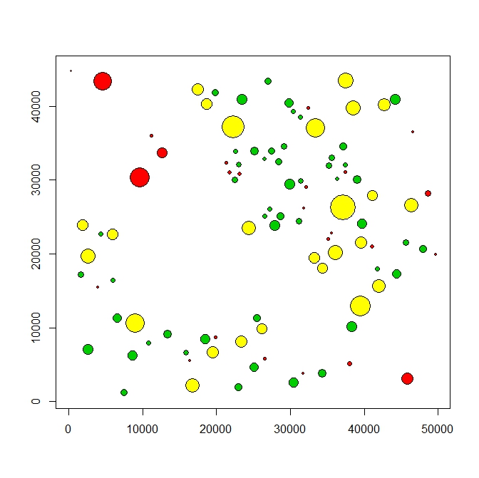
# the following instructions yield a spatial representation of the
# estimated incidences: different colors reflect three different
# classes of incidence values, as defined by the quantiles

plot(x.crd,y.crd,asp=1,xlab="",ylab="",pch=21,col="black",bg=0,cex=sqrt(A*3))

pos1<-which(fitted1 <= quantile(fitted1,0.25))
pos2<-which(fitted1 > quantile(fitted1,0.25) & fitted1 <= quantile(fitted1,0.75))
pos3<-which(fitted1 > quantile(fitted1,0.75))

points(x.crd[pos1],y.crd[pos1],pch=21,bg=2,cex=sqrt(A[pos1]*3))# red
points(x.crd[pos2],y.crd[pos2],pch=21,bg=3,cex=sqrt(A[pos2]*3))# green
points(x.crd[pos3],y.crd[pos3],pch=21,bg=7,cex=sqrt(A[pos3]*3))# yellow

Example 10.4. Basic IFM with rescue effect. One only snapshot.
We estimate the parameters of a basic IFM by using only the presence absence vector “p1” of the reference metapopulation REFMETAPOP. The instructions are as in Example 10.3, apart for the incidence function:

S<-rowSums(edis[,p1>0])

incRE<-function(i, x, y){ (A[i]^x)*S[i]^2/((y^2*A0^x)+(S[i]^2*A[i]^x)) }

LL<- function(x,y) { R = dbinom(p1,1,incRE(1:100,x,y),log = TRUE) -sum(R) }

library(stats4)

fit2 <- mle(LL, start = list(x=0.05, y=0.5), method = "L-BFGS-B", lower = rep(0, 2))

summary(fit2)

Maximum likelihood estimation

Call:
mle(minuslogl = LL, start = list(x = 0.05, y = 0.5), method = "L-BFGS-B", lower = rep(0, 2))

Coefficients:

	Estimate	Std. Error
x	0.1829159	0.2830272
y	0.1354577	0.1511952

-2 log L: 222.9346

param<-coef(fit2)

xhat<-param[1]
yhat<-param[2]

# Then, E and C can be computed

C<-S^2/(S^2+yhat^2)
E<-(1-C)*pmin(A0^xhat/A^xhat,1)

# estimated incidences

fitted2<-incRE(1:100,xhat,yhat)

summary(fitted2)

0.00000.31100.78330.61000.93560.9857

Min.

1st Qu.

Median

Mean

3rd Qu.

Max.

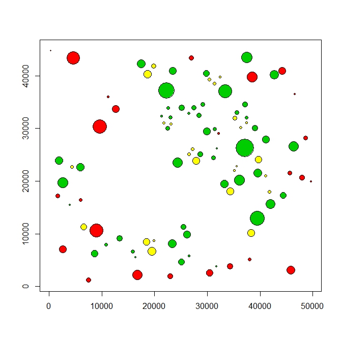
# The following picture has been obtained as in Example 10.3, and the
# colors have the same meaning.

4. Some technicalities

The R instruction mle(LL, start = list(x=0.05, y=0.5), method = "L-BFGS-B", lower = rep(0, 2)) requires a starting point for each variable. Different starting points can give rise to different results, as in Example 10.5.

Example 10.5.
Referring to Example 10.3, two different starting points have been considered:

fit1a <- mle(LL, start = list(x=0.05, y=0.9), method = "L-BFGS-B", lower = rep(0, 2))

summary(fit1a)

Maximum likelihood estimation

Call:
mle(minuslogl = LL, start = list(x = 0.05, y = 0.9), method = "L-BFGS-B", lower = rep(0, 2))

Coefficients:

	Estimate	Std. Error
x	0.087394825	0.033275216
y	0.001088747	0.001620498

-2 log L: 126.881

fit1b <- mle(LL, start = list(x=1.5, y=0.1), method = "L-BFGS-B",
+ lower = rep(0, 2))

Error in optim(start, f, method = method, hessian = TRUE, ...) :
L-BFGS-B needs finite values of 'fn'.

Compared to fit1 of Example 10.3, in the case of fit1a, slightly different estimates have been obtained, but the likelihood values are very close. Then, the two estimated models are substantially equivalent.

In the case of fit1b, the command is not able to provide an answer. An error message is displayed referring to the fact that for some values of x and y, the function ("fn", i.e. LL) we are trying to optimize does not have a finite value. This is because in some cases the argument of the logarithm function (see Eq. (10.2)) can be numerically equal to 0, and an “infinite” value obtained. This problem can be solved by choosing different starting values in start.

As in the case of Examples 10.1 and 10.2, it can be useful to look at a plot of the likelihood function to find suitable starting points.

Example 10.6.
To complete Example 10.3, we provide some instructions to plot the minus-log-likelihood function.

# We define a grid over the domain of the function, that is a set of
# pairs (x,y):

x1<-seq(0,1,by=0.01)
y1<-seq(0,2,by=0.01)

length(x1)

[1] 101

x1[1:10]

[1] 0.00 0.01 0.02 0.03 0.04 0.05 0.06 0.07 0.08 0.09

# and then for each point (x1[k], y1[j]) of the grid we compute the
# value of –LL : these values are stored in a matrix, z

z <- matrix(0,nrow=length(x1), ncol=length(y1))
for(k in 1:length(x1)) {
for(j in 1:length(y1)) { z[k,j]<-LL(x1[k],y1[j]) }
}

persp(x1,y1,-z,phi=20,theta=20,d=10,col="light blue",ticktype="detailed",xlab="x",ylab="y", zlab="- LOG-LIKELIHOOD")

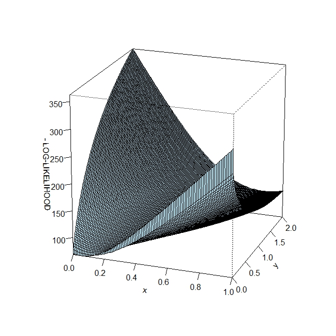
# a useful indication for setting the starting points for the search
# algorithm is the contour plot:

contour(x1,y1,z,col="blue",xlab="x",ylab="y",main="CONTOUR PLOT")

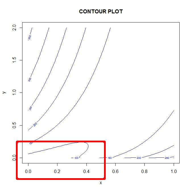
Each line in the contour plot is a level-curve, that is a curve joining all the points (x,y) having the same “z”. As we are searching for a minimum value, the region of interest is the one defined by the lowest level, here 100. Therefore, a suitable choice as start in the mle command is an x value between 0 and about 0.5 and a y value between 0 and about 0.3, or close values.