Model Simulation - Part I
Model Simulation (I)
1. Model Simulation
Before discussing model parameters, we introduce a few examples showing how to simulate metapopulation dynamics following an IFM.
Regardless of the specific IFM model (the basic IFM, the “time dependent” or any of the two models with rescue effect), dynamics simulation (i.e., presence/absence at subsequent times) can be obtained in the following way. For a given parameters set, start the simulation from an initial vector of states (either 0 or 1) of the n local populations. For each time t calculate Si(t), Ci(t) and Ei(t) according to the model-specific formulas, and generate a random number U according to a uniform distribution on (0,1). Finally, determine the population state of patch i at time t+1, xi(t+1), by comparing Ei(t) and Ci(t) to U :
\(x_i(t+1)= \begin{cases} 1,& if\: x_i(t) = 0 \: \: \& \:\:U \le C_i(t)\\ 0,& if\: x_i(t) = 0 \: \: \& \:\:U \gt C_i(t)\\ 0,& if\: x_i(t) = 1 \: \: \& \:\:U \le E_i(t)\\ 1,& if\: x_i(t) = \: \: \& \:\:U \gt E_i(t)\\ \end{cases} \)
Example 7.1. BASIC IFM.
We will consider, as usual, the reference metapopulation of Example 4.1.
We show how to simulate the dynamics of a basic IFM (see Unit 4). Vectors p and p1 are here used as “historical data” to determine the (constant) colonization probability, according to Eqs. (4.5) and (5.1).
DATA<-read.table("REFMETAPOP.txt",header=TRUE)
attach(DATA)
# parameter values
alpha<-1
A0<-0.0004
xhat<-0.05
yhat<-0.005
# extinction probabilities
E<-pmin(A0^xhat/A^xhat,1)
# connectivity and colonization probabilities, based on the mean
# observed occupancy time, pm
d<-dist(cbind(x.crd,y.crd))/1000
edis<-as.matrix(exp(-alpha*d))
edis<-sweep(edis,2,A,"*")
pm<-(p+p1)/2
S<-rowSums(edis[,pm>0])
C<-S^2/(S^2+yhat^2)
# We introduce the function sim1: the argument of sim1 is any
# presence/absence vector of length equal to the metapopulation size
# (100).
# The key element of sim1 is the function runif. runif(1) generates a
# number between 0 and 1 (U)according to the uniform distribution.
# runif(k) generates k numbers.
sim1<-function(o){</p> <p class="formule">o<- o > 0 </p> <p class="formule">if(any(o)){</p> <p class="formule">cond<-ifelse(o,E,C)</p> <p class="formule">o<-ifelse(runif(length(o))<cond,!o,o)</p> <p class="formule">}
as.numeric(o)
}
# the main instruction in the definition of sim1 is
# ifelse(runif(length(o))<cond,!o,o) that compares each of the 100
# values “U” generated by runif to E if the corresponding element of o
# is equal to 1 and to C otherwise.
# One simulation of 10 subsequent years of metapopulation dynamics,
# starting from p1 (see Remark 3.2, Unit 3): we start with a null matrix
# sim; the initial state p1 is assigned to the first column, then by the
# command for a new column, i.e. metapopulation state, is generated from
# the previous one.
#
nt=10;
sim<-matrix(0,nrow=length(p1),ncol=nt+1)
sim[,1]<-p1
sim[1:10,]
[,1] [,2] [,3] [,4] [,5] [,6] [,7] [,8] [,9] [,10] [,11]
[1,] 1 0 0 0 0 0 0 0 0 0 0
[2,] 0 0 0 0 0 0 0 0 0 0 0
[3,] 1 0 0 0 0 0 0 0 0 0 0
[4,] 0 0 0 0 0 0 0 0 0 0 0
[5,] 0 0 0 0 0 0 0 0 0 0 0
[6,] 0 0 0 0 0 0 0 0 0 0 0
[7,] 0 0 0 0 0 0 0 0 0 0 0
[8,] 1 0 0 0 0 0 0 0 0 0 0
[9,] 1 0 0 0 0 0 0 0 0 0 0
[10,] 1 0 0 0 0 0 0 0 0 0 0
for(t in 1:nt) sim[ ,t+1]<-sim1(sim[ ,t])
sim[1:10,]
[,1] [,2] [,3] [,4] [,5] [,6] [,7] [,8] [,9] [,10] [,11]
[1,] 1 0 1 1 0 1 0 1 0 1 0
[2,] 0 1 0 1 0 1 0 1 0 1 0
[3,] 1 0 1 0 1 0 1 0 1 0 1
[4,] 0 1 0 1 0 1 0 1 0 1 0
[5,] 0 1 1 0 1 0 1 0 1 1 1
[6,] 0 1 0 1 1 1 0 1 0 1 0
[7,] 0 1 0 1 0 0 0 1 1 0 1
[8,] 1 0 1 0 1 0 1 1 1 0 1
[9,] 1 0 1 1 1 1 1 0 1 1 0
[10,] 1 0 1 0 1 0 1 0 1 0 1
# Note that if you run these commands on your computer, this
# output and the following picture as well will differ as runif
# generates different values at each run.
# number of occupied sites in each year (i.e., column of sim)
plot(colSums(sim),type="o",lwd=2,xlab="t",ylab="n. occupied sites")
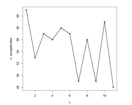
Figure 7.1 shows the effect of considering rescue effect in the case of Example 7.1 by comparing the yearly number of occupied sites, under the two models. This figure has been obtained with the following instructions:
|
plot(colSums(sim),type="o",lwd=2,xlab="t",ylab="n. occupied sites", ylim=c(0,100)) # ylim sets the vertical plot range # simRE is the matrix of simulations obtained by including rescue # effect (see Exercise 7.1) points(colSums(simRE),col="red", type="o", lwd=2,xlab="t",ylab="n. occupied sites", ylim=c(0,100)) # points works like plot, however it allows to add the new graphic to # the previous one text(3,98,labels="RESCUE EFFECT") text(3,48,labels="NO RESCUE EFFECT") |
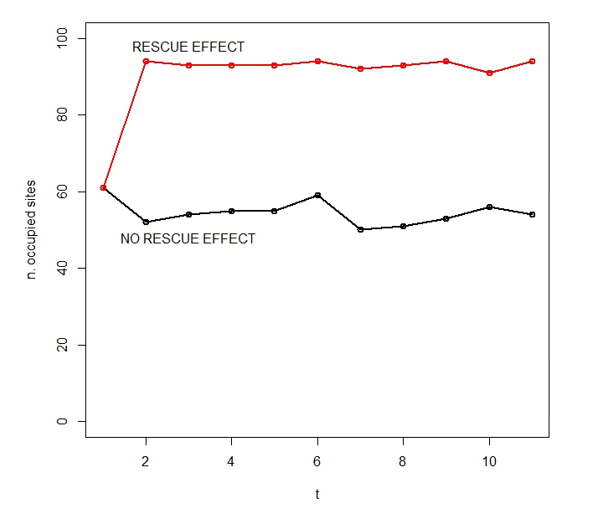
Figure 7.9 – Number of occupied sites in two simulations of the basic IFM with and without rescue effect.
and clearly shows that the number of occupied sites strongly increases by the rescue effect.
Example 7.2. “Time-dependent” IFM.
We now consider the model of Unit 6, without rescue effect (Eq. (6.2)). As both connectivity and colonization probability are not constant, the computation of S and C cannot be carried out in advance, but should be included in the function sim1.
sim1TD<-function(o){</p> <p class="formule">o<- o > 0 </p> <p class="formule">if(any(o)){</p> <p class="formule">S<-rowSums(edis[,o,drop=FALSE])</p> <p class="formule">C<-S^2/(S^2+yhat^2)</p> <p class="formule">cond<-ifelse(o,E,C)</p> <p class="formule">o<-ifelse(runif(length(o))<cond,!o,o)</p> <p class="formule">}
as.numeric(o)
}
The simulated numbers of occupied sites are compared in the following picture. The chain starts at p1. Instructions are as before.
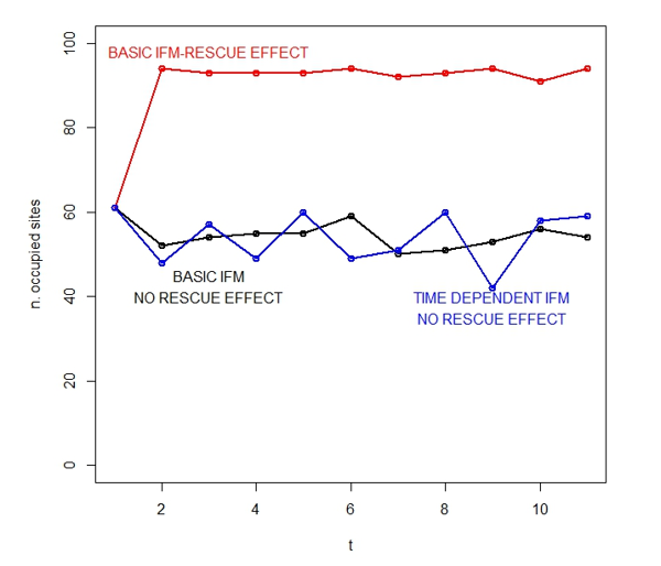
Pictures like Figure 7.1 or the one in Example 7.2 are not sufficient to clearly show the differences among models, as the visual effect is determined by the result of the specific simulation. For instance, the picture of Example 7.2 could suggest that the time-dependent model adds more variability to the yearly number of occupied sites than the basic IFM (excluding rescue effect in both cases). However, another run of sim1TD yields Figure 7.2, where the black and the blue lines are very similar.
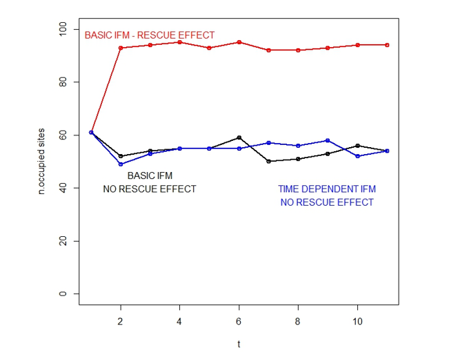
Figure 7.2 - Number of occupied sites in one simulation of the basic IFM with and without rescue effect compared to one simulation of the time-dependent IFM without rescue effect.
More precise information is obtained by averaging over a large number of simulations. By repeating simulations for several times, information on the distributions of the vectors Xt at different times t can also be obtained, as shown in Example 7.3. We discuss this latter issue in the following Section 7.1 and go back to model comparison in Unit 8.