Finite Markov Chains - Part II
SHORT INTRODUCTION TO FINITE MARKOV CHAINS - Part II
SHORT INTRODUCTION TO FINITE MARKOV CHAINS - Part II
Let (Xt )t ≥ 1 be a discrete-time, finite-space, homogeneous first order Markov Chain as introduced in Unit 2.
By the simple Bayes theorem, it can be easily seen that
(3.1)P(X2 = xi) = ∑k=1,…,N P(xk , xi) \(\pi\)(xk)
that is P(X2 = xi) is obtained as the sum over all the ways in which the process can start from X1
and then move onto xi.
| Example 3.1. |
| In the setting of Example 2.2 |
| P(X2 = 1) = P(X2 = 1| X1 = 0) \(\pi\)(0) + P(X2 = 1| X1 = 1) \(\pi\)(1) = 0.50×0.25 + 0.60×0.75 = 0.575. |
Moreover, it follows from (2.3) that P(Xt+1 = xi) can be obtained as a sum of the probabilities
of the possible paths X1 = xk,1 , ... , Xt = xk,t :
P(Xt+1 = xi) = ∑ { \(\pi\)(x<sub>k,1</sub>) P(x<sub>k,1</sub>, x<sub>k,2</sub>) ...
P(x<sub>k,t-1</sub>, x<sub>k,t</sub>) P(x<sub>k,t</sub> , x<sub>i</sub>) : (x<sub>k,1</sub>, ... , x<sub>k,t</sub> ) }.
In matrix notation, regarding π as a row vector, we can write:
(3.2)P(Xt+1 = xi) = ( \(\pi\)Pt )(i)
that is P(Xt+1 = xi) is the i-th element of the vector \(\pi\)Pt, where Pt means the matrix product of P for t times,
and the element pij(t) of Pt gives the probability of arriving at state j after t time steps given that the chain started at state i.
Referring to Example 2.3, Figure 9 shows the probability densities of Xt for t = 1, … , 10 for two different initial distributions,
\(\pi\) as in Example 2.3, and \(\pi\)1. In each picture, each of the colored lines represent P(Xt = xi)
for a given state xi as time t goes from 1 to 10.
It can be clearly seen that these probabilities converges, that is each colored line tends to quickly become horizontal.
Moreover, two curves with the same color in the two pictures converge to the same value,
regardless of the initial probability distribution. That is, for t = 10 we have that
|
This is the core of the final part of this Unit: the concept we are introducing will be particularly relevant for the IFM model.
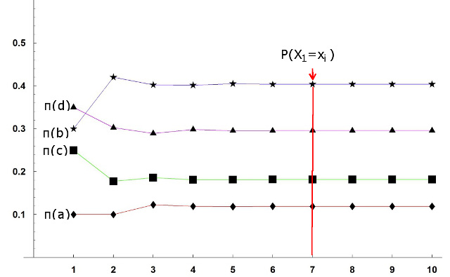
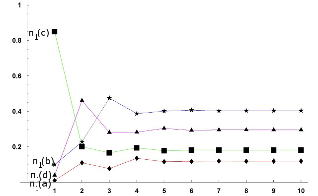
Figure 9 – Referring to Example 2.3, time evolution of the density distribution of Xt according to Eq. (3.2). Starting distribution: \(\pi\) as in Example 2.3 (top) and a different initial distribution \(\pi\)1 assigning a high probability (0.85) of starting from state c (down). The density distribution at time t can be read vertically, as in the case of t=7 at the top.
If the initial distribution is such that
(3.3) P(X2 = xi) = ∑k=1, ...,N P(xk , xi)
\(\pi\)(xk) = \(\pi\)(xi) for any i = 1, ... , N
that is, P(X2 = xi) = P(X1 = xi) for any
i = 1, ... , N, then, by applying Eq. (3.2) we obtain, for any t ≥ 2
(3.4)P(Xt = xi) = \(\pi\)(xi) for any i
that is, the random observations have all the same probability density \(\pi\).
Such a common probability distribution is called
invariant or
equilibrium (this is a term used by Hanski and co-authors) or
stationary
 and
(Xt)t≥1 is a stationary Markov chain.
and
(Xt)t≥1 is a stationary Markov chain.
Example 3.1 shows that there \(\pi\) is not an invariant distribution, as P(X2 = 1) = 0.575 while \(\pi\)(1) = 0.7. In general,
existence and uniqueness of the stationary distribution are not guaranteed.
However for a two-state process (0 and 1), like that of Example 2.2, the (unique) invariant initial distribution
\(\pi\)* can be easily obtained by solving
P(X2 = 1) = P(0, 1) \(\pi\)*(0) +
P(1, 1) \(\pi\)*(1) =
P(0, 1) × (1- \(\pi\)*(1)) + P(1, 1) × \(\pi\)*(1) = \(\pi\)*(1)
that is
\(\pi\)*(1) [1 - P(1, 1) +
P(0, 1) ] = P(0, 1).
As 1 - P(1, 1) = P(1, 0), this means
| (3.5) |
|
|||||||
Of course, this holds true if P(1, 0) + P(0, 1) ≠ 0.
In Example 3.2, \(\pi\)*(1) = 0.5/(0.4+0.5) = 0.56.
We will not deepen insight into the general theory of the invariant distributions,
but we will only consider the invariant distribution for the two-state process,
as Eq. (3.5) will be fundamental in the discussion of the basic IFM in Unit 4.
The cases P(1, 0) = P(0, 1) = 0 and P(1, 0) =
P(0, 1) = 1 will be always excluded.
Asymptotic results.
For the two state process, it can be proved (Norris 1997, Theorem 1.8.3 p. 41) that
P(Xt = 1) → \(\pi\)*(1) as t → +∞
and the probabilities of arriving at 1 in t time steps
(i.e., the elements of the matrix Pt) converges to the invariant distribution as well:
both P(Xt+1 = 1 | X1 = 0) and P(Xt+1 = 1 | X1 = 1) → \(\pi\)*(1) as t → +∞
(and the other conditional probabilities accordingly).
Remark 3.1.
Let (Xt)t≥1 a Markov chain with transition matrix
P and initial distribution \(\pi\).
The Markov property (2.1) yields that conditional on Xt = x, the (future) process (Xt+s)s≥1
is still a Markov chain with initial distribution assigning unit mass to x,
and transition matrix P.
Moreover, it is independent of the random variables X1, ... , Xt. (Norris 1997, Theorem 1.1.2 p. 3).
In other words, if we know that at time t we are at state x,
the future observations follow a Markov chain with the same transition matrix P
and initial probability with unit mass on x (as we are certain about the starting state, x),
regardless of the way in which we arrived at x.
Remark 3.2.
Let x be the starting point, that is X1 = x, and let Tx be the first return time at state x,
that is the first time t > 1 such that Xt = x.
Looking at Example 1, T1 = 3 as (X1, X2, X3) = (1, 0, 1).
If (X1, X2, X3) = (1, 1, 0), then T1 = 2.
If (X1, X2, X3) = (1, 0, 0), then we can only say that T1 should be at least 4.
The return times Tx are random variables taking any integer value.
Then, if an invariant measure \(\pi\)* exists, the expected value of Tx, E(Tx),
is given by 1/\(\pi\)*(x).
For the presence/absence process of Example 2, the mean time between two consecutive "presences"
(mean return time at state 1, starting from 1) is 1/\(\pi\)*(1) = 1/0.56 = 1.78 years,
while the mean time between two consecutive "absences" (mean return time at state 0, starting from 0)
is 1/\(\pi\)*(0) =1/(1-0.56) = 2.27 years.