The incidence Function Model - Part II
The incidence Function Model (II)
1. The basic model, contd.
In Section 4.1 we hypothesized that only one snapshot of data is available, and in Example 4.1 the column "p" only has been considered for representation. Indeed, one only snapshot of data is enough for the computation of connectivity and extinction probabilities, as shown in Example 5.1.
Example 5.1.
We consider again the reference metapopulation of Example 4.1 and we compute extinction and colonization
probabilities based on the vector "p".
DATA<-read.table("REFMETAPOP.txt",header=TRUE)
attach(DATA)
# The following commands yield the computation of connectivity,
# extinction and colonization probabilities.
#
# intra-patches distances, expressed in km (/1000) :
d<-dist(cbind(x.crd,y.crd))/1000
# Note that the previous command do not yield any output. This is
# obtained by the command
# parameter \(\alpha\), here denoted by "alpha", is here fixed to 1:
alpha<-1
# connectivity S is obtained by firstly constructing the matrix edis
# of values exp(-αdik) (see Eq. (4))
edis<-as.matrix(exp(-alpha*d))
# then by adding the area as multiplying term exp(-\(\alpha\)dik)Ak
edis<-sweep(edis,2,A,"*")
# and finally by summing, for each row, the terms corresponding to
# occupied patches, see Eq. (4).
S<-rowSums(edis[,p>0])
# The first 10 connectivity values are
S[1:10]
| 1 | 2 | 3 | 4 | 5 |
| 0.009051098 | 0.267525280 | 0.099883377 | 0.034759202 | 0.108124919 |
| 6 | 7 | 8 | 9 | 10 |
| 0.470139254 | 0.006580590 | 0.323074862 | 0.034888360 | 0.242323462 |
# Colonization probabilities:
C<-S^2/(S^2+yhat^2)
# Let fix parameters A0 (here denoted by “A0”), x (“xhat”) and y
# (“yhat”):
A0<-0.0004 (xhat<-0.05)
[1] 0.05
(yhat<-0.005)
[1] 0.005
# extinction probabilities:
(E<-pmin((A0/A)^xhat,1))
[1] 0.7539049 0.6637643 0.7552373 0.7079112 0.6997523 0.6622258 0.6658542 0.7136843
[9] 0.6735996 0.6467836 0.6725409 0.7146209 0.6640752 0.7235986 0.6820508 0.6961306
[17] 0.7395705 0.7557628 0.6627929 0.6918963 0.6457575 0.6657251 0.7147616 0.6612739
[25] 0.6294102 0.7506815 0.6642616 0.7585497 0.6715268 0.7173304 0.6145489 0.6737645
[33] 0.6215733 0.7004557 0.7706369 0.6660214 0.7484575 0.6859309 0.7429758 0.6407704
[41] 0.6407039 0.6683193 0.7387849 0.7298567 0.6778981 0.6264860 0.6584399 0.7029354
[49] 0.7009214 0.6089256 0.6562716 0.6784673 0.7288610 0.6968343 0.6571807 0.6629583
[57] 0.6674814 0.7347118 0.7329261 0.6835437 0.7128088 0.6671616 0.7372821 0.7505267
[65] 0.7027723 0.7014718 0.6550001 0.6678379 0.7156306 0.7173560 0.7517339 0.6921919
[73] 0.6959897 0.6988516 0.6792371 0.6929424 0.7258438 0.6897501 0.6660901 0.6596272
[81] 0.6579770 0.6446141 0.6824783 0.7209536 0.6539113 0.6523355 0.6545286 0.7185262
[89] 0.6261870 0.6411517 0.6795544 0.7130378 0.6451583 0.6911837 0.7127963 0.6247640
[97] 0.6833305 0.7469326 0.7479725 0.6398044
The situation of Example 4.1 and Example 5.1 reflects quite common situations, however is not unusual to have two or more observations in the course of time at each patch. This case can be encompassed within the basic model, by simply substituting the averaged observations \(\bar{\delta}_i\) (observed mean occupancy time) to \(\delta_i\) in Eq. (4.4)
(5.1)\(M_i=\beta S_i=\beta\sum_{k≠i}\bar\delta_i exp(-\alpha d_{ik}) A_k\)
and then using this averaged connectivity in (4.5) to still obtain a colonization probability based on all the observations collected at each site. Of course, the temporal order of the data is not taken into account.
Example 5.2.
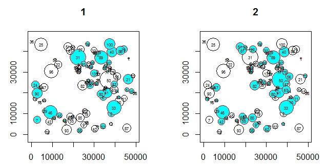
Let us consider again the reference metapopulation of Example 5.1, and now consider both the vectors p and p1.
DATA<-read.table("REFMETAPOP.txt",header=TRUE)
attach(DATA)
sum(p)
[1] 45
sum(p1)
[1] 61
# To plot the two vectors of presence/absence on one plot 2 x 1 with a # square plotting region independent of device size:
op <- par(mfrow = c(1,2), pty="s")
for(k in 1:2){<br>
plot(x.crd,y.crd,asp=1,xlab="",ylab="",cex=sqrt(A*3),<br>
pch=21, col=DATA[,3+k]+1, bg=5*DATA[,3+k],main=k)<br>
text(x.crd,y.crd,labels=c(1:100),cex=0.5,col=1)}
# At end of plotting, reset to previous settings:
par(op)
# as in Example 5.1:
d<-dist(cbind(x.crd,y.crd))/1000
alpha<-1
edis<-as.matrix(exp(-alpha*d))
edis<-sweep(edis,2,A,"*")
A0<-0.0004
xhat<-0.05
yhat<-0.005
E<-pmin(A0^xhat/A^xhat,1)
# Let pm be the mean time occupancy per patch:
(pm<-(p+p1)/2)
[1] 0.5 0.5 0.5 0.5 0.5 0.5 0.5 1.0 0.5 0.5 0.5 0.5 0.5 0.5 0.5 1.0 0.0
[18] 0.5 0.0 0.5 0.5 0.0 1.0 0.5 0.0 0.5 0.5 0.5 0.5 0.5 0.5 0.5 1.0 1.0
[35] 0.0 0.5 0.5 1.0 0.5 1.0 1.0 0.5 0.5 0.5 0.5 1.0 0.5 1.0 0.5 0.5 0.5
[52] 0.5 0.5 0.5 0.5 0.5 0.5 0.0 0.5 0.5 0.5 0.5 1.0 0.5 0.5 1.0 0.5 0.5
[69] 0.5 0.5 0.5 0.5 0.5 0.5 0.5 1.0 1.0 0.0 0.5 1.0 0.5 0.5 0.0 0.5 0.5
[86] 0.5 0.0 0.5 1.0 0.5 0.5 0.5 0.0 0.5 0.5 0.0 1.0 0.5 0.5 0.5
# connectivity and colonization probabilities are computed based on pm
S<-rowSums(edis[,pm>0])
C<-S^2/(S^2+yhat^2)
# and compared with those based on p only
S1<-rowSums(edis[,p>0])
C1<-S1^2/(S1^2+yhat^2)
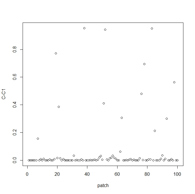
plot(C-C1,xlab=”patch”, ylab=”C-C1”)
length(which(C-C1>0))
[1] 100
# for all the patches, the new colonization probabilities are higher
# than the old ones, as expected. Indeed, it is sufficient for a patch
# to be occupied one time only to contribute to S and then to C.
# The following instruction pinpoints the patches for which the
# difference is greater than 0.1
DATA[which(C-C1>0.1),]
| x.crd | y.crd | A | p | p1 | |
| 7 | 2561.576 | 7068.673 | 1.3629405 | 1 | 0 |
| 19 | 26177.833 | 9908.575 | 1.4945247 | 0 | 0 |
| 21 | 46432.106 | 26569.624 | 2.5157717 | 1 | 0 |
| 38 | 22956.360 | 1950.972 | 0.7524065 | 1 | 1 |
| 51 | 17404.085 | 42278.952 | 1.8213241 | 0 | 1 |
| 52 | 34315.750 | 3846.805 | 0.9364439 | 1 | 0 |
| 63 | 19812.524 | 8696.669 | 0.1775768 | 1 | 1 |
| 76 | 27000.395 | 43374.797 | 0.6139285 | 1 | 1 |
| 78 | 7484.348 | 1160.344 | 0.6733251 | 0 | 0 |
| 83 | 25481.567 | 11302.356 | 0.8323061 | 0 | 0 |
| 85 | 23334.392 | 8117.678 | 1.9574174 | 0 | 1 |
| 93 | 16795.340 | 2119.424 | 2.5629134 | 0 | 0 |
| 98 | 26539.666 | 5785.241 | 0.1369089 | 1 | 0 |