Parameter Estimation - Part II
| Site: | LifeWatch ERIC Training Platform |
| Course: | Spatially explicit metapopulation model - Incidence Function Model |
| Book: | Parameter Estimation - Part II |
| Printed by: | Guest user |
| Date: | Tuesday, 15 September 2026, 2:26 PM |
Description
Parameter Estimation (II)
1. Some estimation issues.
In all the examples of Unit 10 we based the estimation procedure on only one presence/absence vector. This has played a fundamental role into the construction of the R code for maximum likelihood estimation. Indeed, the likelihood function is defined as
LL<- function(x,y) {<br>
R = dbinom(o,1,inc(1:length(o),x,y),log = TRUE)<br>
-sum(R)<br>
}
where “o” is a presence/absence vector, like “p” or “p1” in our reference metapopulation REFMETAPOP. The function LL uses the function dbinom, requiring a vector of integers as first argument (see Remark 10.1). Then, this function cannot be directly used as it is if the observed mean occupancy time is used, as in Eq. (5.1) and Example 5.2. However, only a slight modification is required: we only need to consider a longer presence/absence vector, the vector obtained by collecting all the vectors together. Indeed, as mentioned in Unit 5, the temporal order of the data is not taken into account, and the likelihood becomes
| (11.1) | \(J_1^{\delta_{11} + \delta_{21}}(1-J_1)^{1-(\delta_{11} + \delta_{21})}\) x ... x \(J_n^{\delta_{1n} + \delta_{2n}}(1-J_n)^{1-(\delta_{1n} + \delta_{2n})}\) |
in the case of two observations per patch (and analogously for more than 2). This requires some simple code gimmick.
Example 11.1. Basic IFM, with more than one snapshot.
We refer to REFMETAPOP, as usual.
pm<-(p+p1)/2 S<-rowSums(edis[,pm>0]) p2<-c(p,p1) length(p2)
[1] 200
# for each presence/absence vector inc should be called, in order to
# match each patch observation with the right area and connectivity.
# Be aware to follow the same order in collecting the vectors as in p2
LL<- function(x,y) {<br>
R = dbinom(p2,1,c(inc(1:length(p),x,y),inc(1:length(p1),x,y)),log = TRUE)<br>
-sum(R)<br>
}
library(stats4)
fit <- mle(LL, start = list(x=0.03, y=0.01), method = "L-BFGS-B", lower = rep(0, 2))
summary(fit)
Maximum likelihood estimation
Call:
mle(minuslogl = LL, start = list(x = 0.03, y = 0.01), method = "L-BFGS-B", lower = rep(0, 2))
Coefficients:
| Estimate | Std. Error | |
| x | 0.04653337 | 0.02160148 |
| y | 0.02134258 | 0.01323335 |
-2 log L: 254.3851
Example 11.2. The boundary problem.
As explicitly mentioned in Example 10.3, the optimization problem we are considering is a constrained problem,
as parameters x and y should be positive.
In this kind of problems, it can occur that the optimum belongs to the boundary that is, either \(\hat{x}\) or \(\hat{y}\).
The R instruction mle takes constraint into account by the option lower = rep(0, 2)
(equivalent to lower = c(0,0)).
However, the behavior of the log-likelihood function on the boundary domain can be explicitly checked, by fixing x = 0
and searching for the minimizing value of y,
fit1 <- mle(LL, start = list(x=0.03, y=0.01), fixed=list(x=0),
method = "L-BFGS-B", lower = rep(0, 2))
summary(fit1)
Maximum likelihood estimation
Call:
mle(minuslogl = LL, start = list(x = 0.03, y = 0.01), method = "L-BFGS-B", fixed = list(x = 0), lower = rep(0, 2))
Coefficients:
| Estimate | Std. Error | |
| y | 0.01287862 | 0.008939929 |
-2 log L: 259.3108
and viceversa:
fit2 <- mle(LL, start = list(x=0.03, y=0.01), fixed=list(y=0),
method = "L-BFGS-B", lower = rep(0, 2))
summary(fit2)
Maximum likelihood estimation
Call:
mle(minuslogl = LL, start = list(x = 0.03, y = 0.01), method = "L-BFGS-B", fixed = list(y = 0), lower = rep(0, 2))
Coefficients:
| Estimate | Std. Error | |
| x | 0.01625944 | 0.01871206 |
-2 log L: 276.5023
It can be easily seen that both the minus 2 x log-likelihood values are higher than the optimum value of Example 11.1, and therefore the minimum is reached out of the boundaries, as stated in Example 11.1.
Example 11.3. The basic IFM with rescue effect: more than one snapshot.
pm<-(p+p1)/2
S<-rowSums(edis[,pm>0])
# As in Example 10.4:
incRE<-function(i, x, y){<br>
(A[i]^x)*S[i]^2/((y^2*A0^x)+(S[i]^2*A[i]^x))<br>
}
# As in Example 11.1:
p2<-c(p,p1)
LL<- function(x,y) {<br>
R = dbinom(p2,1,c(incRE(1:length(p),x,y),incRE(1:length(p1),x,y)),log = TRUE)<br>
-sum(R)<br>
}
fit1 <- mle(LL, start = list(x=0.3, y=0.005), method = "L-BFGS-B", lower = rep(0, 2))
summary(fit1)
Maximum likelihood estimation
Call:
mle(minuslogl = LL, start = list(x = 0.3, y = 0.005), method = "L-BFGS-B",
lower = rep(0, 2))
Coefficients:
| Estimate | Std. Error | |
| x | 0.727931 | 0.1609262 |
| y | 2.646930 | 1.6099283 |
-2 log L: 334.8636
2. Parameterization of the basic IFM with rescue effect: an interpretation by regression
In the related literature, the estimation method illustrated in this and in the previous Unit for the IFM model is referred to as nonlinear regression (H94; Moilanen, 1999). It is beyond the aim of this course to discuss this topic. However, in the case of the basic IFM with rescue effect something similar to the usual linear regression can be done. As this has an interesting implication for the IFM parameterization, we will sketch out the logistic model and the relationship with Unit 10 and Section 11.1. In the usual linear regression model, parameters are estimated by minimizing the differences (or residuals) between the observed response and the model expected values, as summarized in Figure 11.1 (that is, the regression line is determined by the ordinary least square method).
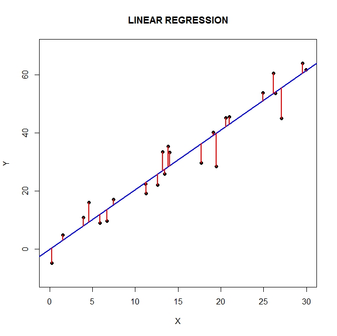
Figure 11 - Scatter plot, regression line (blue) of Y on X and residuals (vertical red bars).
The estimated linear regression provides the expected value of the dependent variable Y, conditional to the dependent variable X=u, E(Y | X=u). For a 0-1 response variable, like presence/absence, this expected value E(Y | X = u) coincides with the (conditional) success probability P(Y = 1 | X = u). Let \(\theta\)(u) = P(Y = 1 | X = u). In the logistic model, it is assumed that
| (11.2) | \[\theta(u)=\frac{e^{\beta_0+\beta_1u}}{1+e^{\beta_0+\beta_1u}}\] |
and therefore, the logit transformation
| (11.3) | \[g(u)=ln\frac{\theta(u)}{1-\theta(u)}=\beta_0+\beta_1u\] |
yields to express a transformation of E(Y | X = u) as linearly dependent from unknown parameters (from which the name of generalized linear model). Of course, k ≤ 1 dependent variables can be considered, yielding the last member of (11.3) to be in the form \(\beta_0+\sum_{j=1}^k\beta_ju_j\)
For the logistic model, the maximum likelihood method applied in Unit 10 and in Section 11.1 is the “equivalent” of the least square method. By proceeding as in Section 10.2 it is easy to prove that parameter estimation is indeed obtained by the minimization of
| (11.4) | \[-\sum_{i=1}^n\{y_iln[\theta(u_i)]+(1-y_i)ln[1-\theta(u_i)]\}\] |
that is, by minimizing a comparison between the observed presence/absence data (\(y_i\)) and the expected presence/absence \(\theta(u_i)\).
The similarity between (11.4) and (10.2) is self-evident. Moreover, we know from Eq. (4.1) that for the basic IFM, the expected presence/absence \(\theta(u_i)\) is given by the incidence \(J_i\) of Eq. (10.3) and Eq. (10.4). Therefore, we only need to check if \(J_i\) can be expressed as in (11.2) or, alternatively, if \(ln (J_i / 1- J_i)\) is a linear combination of the unknown parameters and the dependent variable (u), as in Eq. (11.3).
We firstly consider Eq(10.4) and prove that Eq. (11.3) holds true.
\(1-J_i =\frac {A_0^xy^2/S_i^2A_i^x}{1+A_0^xy^2/S_i^2A_i^x}\) and then \(\frac{J_i}{1-J_i}=\frac{A_i^xS_i^2}{A_0^xy^2}\) , so that \(ln\frac{A_i^xS_i^2}{A_0^xy^2}=xln(\frac{A_i}{A_0})-2lny+2lnS_i\).
Therefore, by considering as independent variables the patch area and the patch connectivity, and naming \(\beta_0= -2 lny\), \(\beta_1=x\), and \(\beta_2=2\) we obtain
| (11.5) | \[g(A_i,S_i)=\beta_0+\beta_1ln(\frac{A_i}{A_0})+\beta_2lnS_i\] |
It can be clearly seen that the unknown parameters x and y can be estimated by regressing the presence/absence data (response) on the (scaled) patch area and the connectivity (independent variables) to estimate the unknown parameters \(\beta_0\) and \(\beta_1\). From the estimated values of \(\beta_0\) and \(\beta_1\) we can go back to x and y (\(y = exp(-\beta_0/2)\)). Note that as \(\beta_1=x\), then \(\beta_1\gt0\), while \(\beta_0\) can be any real number.
Example 11.4. The basic IFM with rescue effect: implementing logistic regression by R.
As in Example 10.4, we estimate the parameters of a basic IFM by using only the presence absence vector “p1” of the reference metapopulation REFMETAPOP.
S<-rowSums(edis[,p1>0])
# the command for fitting a generalized linear model is glm
mod1<-glm(p1~offset(2*log(S))+log(A/A0),family=binomial)
# by specifying family=binomial, the logistic regression is carried
# out. The fact that \(\beta_2\) = 2 in Eq. (11.5) is specified by offset.
summary(mod1) # we will not discuss all the content of the output
Call:
glm(formula = p1 ~ offset(2 * log(S)) + log(A/A0), family = binomial)
Deviance Residuals:
| Min | 1Q | Median | 3Q | Max |
| -2.8370 | -0.8695 | 0.3104 | 0.7377 | 4.3226 |
Coefficients:
| Estimate | Std. Error | z value | Pr(>|z|) | ||
| (Intercept) | 4.0009 | 2.2398 | 1.786 | 0.0741 | . |
| log(A/A0) | 0.1826 | 0.2839 | 0.643 | 0.5202 | * |
---
Signif. codes: 0 '***' 0.001 '**' 0.01 '*' 0.05 '.' 0.1 ' ' 1
(Dispersion parameter for binomial family taken to be 1)
| Null deviance: | 223.34 on 99 degrees of freedom |
| Residual deviance: | 222.93 on 98 degrees of freedom |
AIC: 226.93
Number of Fisher Scoring iterations: 5
Please, note that the regression signed in red (*) is not significant! That is, p1 does not contain enough evidence to state that the presence of the species in any patch depends on the patch area. However, assessing statistical significance is not here the main aim, as this dependence is directly hypothesized in Eq. (5.2).
Then, from the estimated betas values we go back to x and y, regardless of the significance of the regression model.
(beta<-coef(mod1))
| (Intercept) | log(A/A0) |
| 4.0008854 | 0.1825774 |
# in the notation of Eq. (11.5), \(\beta_0 = beta[1]\) and \(\beta_1 = beta[2]\)
# therefore
(xhat<-beta[2])
log(A/A0)
0.1825774
(yhat<-exp(-beta[1]/2))
| (Intercept) |
| 0.1352754 |
Please, note that the estimated values xhat and yhat coincide (apart from numerical approximation) with those directly obtained in Example 10.4 by maximum likelihood estimation.
The regression analysis can be carried out in the case of more than one snapshot, as in Example 11.3.
pm<-(p+p1)/2
S<-rowSums(edis[,pm>0])
# As before, we need to specify that two year of data are used. This
# is done by cbind, which creates a matrix 100x2 where for each patch
# the first column contains the number of successes in the 2 trials,
# and the second column the number of failures.
cbind(p+p1,2-p-p1)[1:10,]
| [,1] | [,2] | |
| [1,] | 1 | 1 |
| [2,] | 1 | 1 |
| [3,] | 1 | 1 |
| [4,] | 1 | 1 |
| [5,] | 1 | 1 |
| [6,] | 1 | 1 |
| [7,] | 1 | 1 |
| [8,] | 2 | 0 |
| [9,] | 1 | 1 |
| [10,] | 1 | 1 |
mod2<-glm(cbind(p+p1,2-p-p1)~offset(2*log(S))+log(A/A0),
family=binomial)
Warning message:
glm.fit: fitted probabilities numerically 0 or 1 occurred
# the warning message tells us that some of the estimated incidences
# (the fitted probabilities) can be equal to either 0 or 1.
summary(mod2)
Call:
glm(formula = cbind(p + p1, 2 - p - p1) ~ offset(2 * log(S)) +
log(A/A0), family = binomial)
Deviance Residuals:
| Min | 1Q | Median | 3Q | Max |
| -2.3433 | -0.7996 | -0.0674 | 0.7902 | 3.4166 |
Coefficients:
| Estimate | Std. Error | z value | Pr(>|z|) | ||
| (Intercept) | -1.9467 | 1.2165 | -1.600 | 0.11 | |
| log(A/A0) | 0.7279 | 0.1609 | 4.523 | 6.09e-06 | *** |
---
Signif. codes: 0 '***' 0.001 '**' 0.01 '*' 0.05 '.' 0.1 ' ' 1
(Dispersion parameter for binomial family taken to be 1)
| Null deviance: | 155.61 on 99 degrees of freedom |
| Residual deviance: | 135.24 on 98 degrees of freedom |
AIC: 239.05
Number of Fisher Scoring iterations: 5
Please, note that the regression (***) is strongly significant! That is, by taking into account both the snapshots "p" and "p1", there is enough evidence to state that the presence of the species in a patch depends on the patch area.
As before, it can be easily seen that the estimated parameters coincide with those obtained in Example 11.3.
Finally, we compare the estimated incidences:
incidences1<-fitted(mod1)
summary(incidences1)
| Min. | 1st Qu. | Median | Mean | 3rd Qu. | Max. |
| 0.0000 | 0.3110 | 0.7833 | 0.6100 | 0.9357 | 0.9857 |
incidences2<-fitted(mod2)
summary(incidences2)
| Min. | 1st Qu. | Median | Mean | 3rd Qu. | Max. |
| 0.0000 | 0.2565 | 0.6169 | 0.5300 | 0.8016 | 0.9282 |
For the basic IFM without rescue effect, it is not possible to obtain an equation similar to Eq. (11.5). Indeed, from Eq. (10.3) we obtain
\(\frac{J_i}{1-J_i}=\frac{A_i^xS_i^2}{A_0^xy^2+A_0^xS_i^2}\) so that \(ln\frac{A_i^xS_i^2}{A_0^xy^2+A_0^xS_i^2}=xln\bigg(\frac{A_i}{A_0}\bigg) + ln\bigg(\frac{S_i^2}{y^2+S_i^2}\bigg)\)
where connectivity Si and parameter y cannot be separated as in Eq. (11.5).