Parameter Estimation - Part I
3. Basic IFM parameterization
Let us refer to Example 10.1. The assumptions of the basic model described in Unit 4, possibly modified by Eq. (5.2) to include rescue effect, allows us to consider the n patches as n coins: the main difference is that each patch has his own “success” probability, expressed by the incidence Ji of Eq. (4.1).
For the sake of simplicity, we firstly consider the case of one only snapshot of data. Referring to Example 10.1, this is equivalent to consider 5 coins with five eventually different probabilities θi, and only one flip for each coin. This leads to P(H,T,T,T,H) = θ1 (1- θ2) (1- θ3) (1- θ4) θ5.
For the IFM, this means that the likelihood function L can be expressed as:
(10.1)\(L(x,y│δ_1,…,δ_n )= J_1^{δ_1}(1-J_1)^{1-δ_1}×… × J_n^{δ_n}(1-J_n)^{1-δ_n} \)
where the usual Bernoulli notation θu (1- θ)1-u = θ if u = 1 and θu (1- θ)1-u = 1-θ if u = 0 is introduced.
Remark 10.1 Bernoulli distribution with R.
The Bernoulli distribution is a special case of a Binomial distribution, with one trial only.
The density of the Binomial distribution with K trials and success probability θ can be computed by R with the following instruction
dbinom(u,K,\(\theta\)) # for each u = 0,1,…,K
For instance, the probability of 2 successes in 5 trials with probability of success in each trial equal to 0.3 is
dbinom(2,5,0.3)
[1] 0.3087
For K=1, dbinom gives the Bernoulli density \(\theta^u(1-\theta)^{1-u}\) (and then u = 0, 1).
To obtain one or more random coin tossing outputs, with success probability \(\theta\) we need the command rbinom(k,1,\(\theta\))
rbinom(1,1,0.58)
[1] 1
rbinom(7,1,0.58)
[1] 0 1 0 1 0 0 0
that is, the function rbinom simulates the results of one or 7 coin flips respectively, for a coin with head probability equal to 0.58.
For optimization, it is very useful to consider the log-likelihood function
(10.2)\(LL(x,y│δ_1,…,δ_n )=∑_{i=1}^n{(δ_i ln[(J_i (x,y)]+(1-δ_i)ln[1-(J_i (x,y)])}\)where the dependence of the incidences on the unknown parameters x and y has been made explicit. Please, note that LL is a negative function, as Ji(x,y) < 1.
By Eq. (4.2) and Eq. (4.5), Ji can be explicitly expressed as
(10.3)\(J_i=\biggl\{{1+[1+\frac{y^2}{S_i^2 }]\frac{(A_0^x)}{(A_i^x )}}\biggr\}^{-1}\)If the rescue effect is taken into account and Eq. (5.2) is applied, then
(10.4)\(J_i= (1+\frac{A_0^x}{A_i^x}\frac{y^2}{S_i^2})^{-1} \)where in both Eq.(10.3) and Eq. (10.4) A0 is assumed to be smaller than the smallest patch of the metapopulation Traditionally, any optimization problem can be formulated in terms of finding the minimum of a given function. This is why the ML estimates will be computed by minimization of the minus-likelihood, or the minus-log-likelihood.
Example 10.3. Basic IFM, one only snapshot.
We estimate the parameters of a basic IFM by using only the presence absence vector “p1” of the reference metapopulation REFMETAPOP.
A0<-0.0004
alpha<-1
d<-dist(cbind(x.crd,y.crd))/1000
edis<-as.matrix(exp(-alpha*d))
edis<-sweep(edis,2,A,"*")
S<-rowSums(edis[,p1>0])
# the following duty function inc1 is introduced
inc1<-function(i, x, y){<br /> (A[i]^x)*S[i]^2/((A0^x)*(S[i]^2+y^2))<br /> }
# and then the incidence function of Eq.(10.3)can be written as
inc<-function(i,x,y){<br /> inc1(i,x,y)/(1+inc1(i,x,y))<br /> }
# The negative log-likelihood function is
LL<- function(x,y) {<br /> R = dbinom(p1,1,inc(1:100,x,y),log = TRUE)<br /> -sum(R)<br /> }
# where dbinom is the binomial density "\(\theta_u(1-\theta)^{1-u}\)". See Remark 10.1.
# the minimization of the negative log-likelihood function can be
# carried out in a numerical way thanks to the R package stats4, that
# contains functions for statistical calculations and random number
# generation. The call of an R package is obtained with the command
# library(package name)
library(stats4)
fit1 <- mle(LL, start = list(x=0.05, y=0.5), method = "L-BFGS-B", lower = rep(0, 2))
# where start is the list of the starting values for the optimization
# algorithm, method selects a numerical optimization method suitable
# for optimization of a function of two or more variables and lower
# defines the constraints on x and y, that are positive values.
summary(fit1)
# shows estimated parameters and (two-times) the log-likelihood
# maximum value (-126.7885).
Maximum likelihood estimation
Call:
mle(minuslogl = LL, start = list(x = 0.05, y = 0.5), method = "L-BFGS-B", lower = rep(0, 2))
Coefficients:
| Estimate | Std. Error | |
| x | 0.075555187 | 0.031313250 |
| y | 0.001220821 | 0.001482456 |
-2 log L: 126.7885
param<-coef(fit1)
xhat<-param[1]
yhat<-param[2]
# Then, E and C can be computed as usual
E<-pmin(A0^xhat/A^xhat,1) C<-S^2/(S^2+yhat^2)
# estimated incidences
fitted1<-inc(1:100,xhat,yhat)
summary(fitted1)
| Min. | 1st Qu. | Median | Mean | 3rd Qu. | Max. |
| 0.0000 | 0.6184 | 0.6356 | 0.5987 | 0.6502 | 0.6790 |
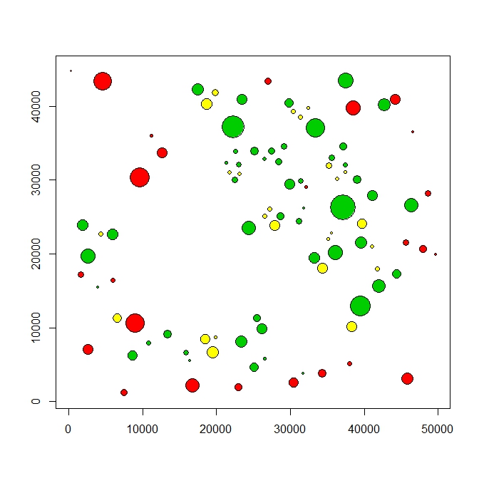
# the following instructions yield a spatial representation of the
# estimated incidences: different colors reflect three different
# classes of incidence values, as defined by the quantiles
plot(x.crd,y.crd,asp=1,xlab="",ylab="",pch=21,col="black",bg=0,cex=sqrt(A*3))
pos1<-which(fitted1 <= quantile(fitted1,0.25))
pos2<-which(fitted1 > quantile(fitted1,0.25) & fitted1 <= quantile(fitted1,0.75))
pos3<-which(fitted1 > quantile(fitted1,0.75))
points(x.crd[pos1],y.crd[pos1],pch=21,bg=2,cex=sqrt(A[pos1]*3))# red
points(x.crd[pos2],y.crd[pos2],pch=21,bg=3,cex=sqrt(A[pos2]*3))# green
points(x.crd[pos3],y.crd[pos3],pch=21,bg=7,cex=sqrt(A[pos3]*3))# yellow
Example 10.4. Basic IFM with rescue effect. One only snapshot.
We estimate the parameters of a basic IFM by using only the presence absence vector “p1” of the reference metapopulation REFMETAPOP. The instructions are as in Example 10.3, apart for the incidence function:
S<-rowSums(edis[,p1>0])
incRE<-function(i, x, y){<br /> (A[i]^x)*S[i]^2/((y^2*A0^x)+(S[i]^2*A[i]^x))<br /> }
LL<- function(x,y) {<br /> R = dbinom(p1,1,incRE(1:100,x,y),log = TRUE)<br /> -sum(R)<br /> }
library(stats4)
fit2 <- mle(LL, start = list(x=0.05, y=0.5), method = "L-BFGS-B", lower = rep(0, 2))
summary(fit2)
Maximum likelihood estimation
Call:
mle(minuslogl = LL, start = list(x = 0.05, y = 0.5), method = "L-BFGS-B", lower = rep(0, 2))
Coefficients:
| Estimate | Std. Error | |
| x | 0.1829159 | 0.2830272 |
| y | 0.1354577 | 0.1511952 |
-2 log L: 222.9346
param<-coef(fit2)
xhat<-param[1]
yhat<-param[2]
# Then, E and C can be computed
C<-S^2/(S^2+yhat^2)
E<-(1-C)*pmin(A0^xhat/A^xhat,1)
# estimated incidences
fitted2<-incRE(1:100,xhat,yhat)
summary(fitted2)
| Min. | 1st Qu. | Median | Mean | 3rd Qu. | Max. |
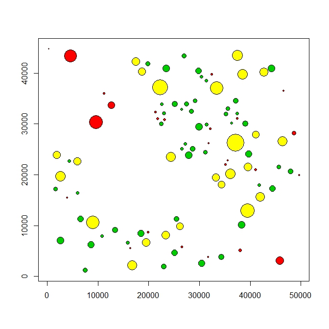
# The following picture has been obtained as in Example 10.3, and the
# colors have the same meaning.