Case study: the Po River Delta - Case study: il delta del fiume Po
| Site: | LifeWatch ERIC Training Platform |
| Course: | Introduction to partitioning and mixed models for biodiversity analysis in R |
| Book: | Case study: the Po River Delta - Case study: il delta del fiume Po |
| Printed by: | Guest user |
| Date: | Tuesday, 15 September 2026, 2:22 PM |
Description
Case study: the Po River Delta - Case study: il delta del fiume Po
Biodiversity partition of the Po River Delta data
In this section we develop a first part of the analysis of the Po River Delta case study. The dataset was collected at 23 monitoring stations grouped in 10 lagoons divided into 3 systems of lagoons (Goro, Fattibello and Comacchio) in the Po River Delta (Northern Adriatic Sea). More specifically the data concern benthic macroinvertebrates collected from monitoring stations presenting from one to three dominant habitat types, defined by a factorial classification of sediment granulometry (sand, mud) and vegetation cover/type (without vegetation, submerged macrophytes, emerged macrophytes and macroalgae) as in Basset et al. (2008b). In every lagoon, field sampling campaigns were performed with one to three monitoring stations per habitat type. Here we consider a hierarchy of multiple spatial scales, with stations nested into lagoons nested into systems. We are interested in verifying how biodiversity changes at different spatial scales and with the order of the diversity, giving decreasing importance to rare species.
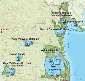
Figure 1: The Po River Delta area
First of all we need to read data from csv files. A faunistic table with densities of individuals as abundance measure and an environmental matrix are available in two files:
> delta=read.table("delta1.csv",header=T,sep=";",row.names=1)
> env=read.table("env1.csv",header=T,sep=";",row.names=1)
> str(delta)
'data.frame': 47 obs. of 23 variables:
$ Fattibello.1 : num 1.05 98.52 5409.41 0 24.31 ...
$ Fattibello.2 : num 0 9.72 105.58 0 5.09 ...
$ Fattibello.3 : num 0 57.9 0 0 3.7 ...
$ Fattibello.4 : num 0 2.78 2.32 0 0 ...
$ Goro.scanno.5 : num 2.32 0 152.35 50.01 7.41 ...
$ Goro.scanno.6 : num 0 49.1 294.5 1477.1 0 ...
$ Goro.scanno.7 : num 0 0 66.7 1784.2 0 ...
$ Smarlacca.8 : num 1077 0 1930 0 0 ...
$ Smarlacca.9 : num 0 103 41305 0 0 ...
$ Taglio.della.Falce.10: num 0 0.694 50.694 0 0 ...
$ Taglio.della.Falce.11: num 0 0 1812 0 0 ...
$ Valle.Campo.12 : num 0 38.6 795.2 0 0 ...
$ Valle.Campo.13 : num 0 0 6.03 0 0 ...
$ Valle.di.Giralda.14 : num 0 0 2548 0 0 ...
$ Valle.di.Gorino.15 : num 0 0 29.17 2.78 0 ...
$ Valle.di.Gorino.16 : num 0 0 4260 0 0 ...
$ Valle.di.Gorino.17 : num 0 1.85 163 0 26.86 ...
$ Valle.di.Gorino.18 : num 0 0 107.43 0 8.34 ...
$ Valle.di.Goro.19 : num 0 2.32 308.86 0 6.48 ...
$ Valle.di.Goro.20 : num 0 5.09 0 0 43.99 ...
$ Valle.di.Goro.21 : num 0 0 107.43 0 8.34 ...
$ Valle.Magnavacca.22 : num 0 0 3751 0 0 ...
$ Valle.Spavola.23 : num 0 42.1 3063.1 0 22.7 ...
> str(env)
'data.frame': 23 obs. of 5 variables:
$ System : Factor w/ 3 levels "Comacchio","Fattibello",..: 2 2 2 2 3 3 3 1 1 3 ...
$ Lagoon : Factor w/ 10 levels "Fattibello","Goro scanno",..: 1 1 1 1 2 2 2 3 3 4 ...
$ Vegetation: Factor w/ 4 levels "emacroph","macroa",..: 2 3 3 3 3 3 3 4 4 1 ...
$ Sediment : Factor w/ 2 levels "mud","sand": 1 1 1 1 2 2 2 1 1 1 ...
$ Station : int 1 2 3 4 5 6 7 8 9 10 ...
We now build the meta-community with communities defined at the mostly local spatial scale, i.e. at the monitoring station level.
> require(entropart)
We let the weights be proportional to the total abundance in each site
> delta.mc1=MetaCommunity(delta,apply(delta,2,sum))
> summary(delta.mc1)
Meta-community (class 'MetaCommunity') made of 444401.8 individuals in 23 communities and 47 species.
Its sample coverage is 1
Community weights are:
| Fattibello.1 | Fattibello.2 | Fattibello.3 | Fattibello.4 | Goro.scanno.5 |
| 0.088027504 | 0.003114463 | 0.012038978 | 0.010219690 | 0.011794114 |
| Goro.scanno.6 | Goro.scanno.7 | Smarlacca.8 | Smarlacca.9 | Taglio.della.Falce.10 |
| 0.021810619 | 0.021438634 | 0.082843290 | 0.279010936 | 0.004723890 |
| Taglio.della.Falce.11 | Valle.Campo.12 | Valle.Campo.13 | Valle.di.Giralda.14 | Valle.di.Gorino.15 |
| 0.057935475 | 0.049738592 | 0.015635579 | 0.109373513 | 0.004734829 |
| Valle.di.Gorino.16 | Valle.di.Gorino.17 | Valle.di.Gorino.18 | Valle.di.Goro.19 | Valle.di.Goro.20 |
| 0.063795908 | 0.014026024 | 0.018809731 | 0.007981528 | 0.008374352 |
| Valle.di.Goro.21 | Valle.Magnavacca.22 | Valle.Spavola.23 | ||
| 0.018809731 | 0.066152821 | 0.029609801 |
Community sample numbers of individuals are:
| Fattibello.1 | Fattibello.2 | Fattibello.3 | Fattibello.4 | Goro.scanno.5 |
| 39119.584 | 1384.073 | 5350.144 | 4541.649 | 5241.326 |
| Goro.scanno.6 | Goro.scanno.7 | Smarlacca.8 | Smarlacca.9 | Taglio.della.Falce.10 |
| 9692.679 | 9527.368 | 36815.710 | 123992.972 | 2099.306 |
| Taglio.della.Falce.11 | Valle.Campo.12 | Valle.Campo.13 | Valle.di.Giralda.14 | Valle.di.Gorino.15 |
| 25746.631 | 22103.922 | 6948.480 | 48605.790 | 2104.167 |
| Valle.di.Gorino.16 | Valle.di.Gorino.17 | Valle.di.Gorino.18 | Valle.di.Goro.19 | Valle.di.Goro.20 |
| 28351.018 | 6233.191 | 8359.079 | 3547.006 | 3721.577 |
| Valle.di.Goro.21 | Valle.Magnavacca.22 | Valle.Spavola.23 | ||
| 8359.079 | 29398.435 | 13158.650 |
Community sample coverages are:
| Fattibello.1 | Fattibello.2 | Fattibello.3 | Fattibello.4 | Goro.scanno.5 |
| 0.9999233 | 1.0000000 | 0.9998127 | 0.9997796 | 0.9996175 |
| Goro.scanno.6 | Goro.scanno.7 | Smarlacca.8 | Smarlacca.9 | Taglio.della.Falce.10 |
| 0.9998968 | 0.9996847 | 1.0000000 | 1.0000000 | 1.0000000 |
| Taglio.della.Falce.11 | Valle.Campo.12 | Valle.Campo.13 | Valle.di.Giralda.14 | Valle.di.Gorino.15 |
| 1.0000000 | 1.0000000 | 1.0000000 | 1.0000000 | 1.0000000 |
| Valle.di.Gorino.16 | Valle.di.Gorino.17 | Valle.di.Gorino.18 | Valle.di.Goro.19 | Valle.di.Goro.20 |
| 1.0000000 | 0.9996785 | 0.9998802 | 0.9997176 | 0.9994603 |
| Valle.di.Goro.21 | Valle.Magnavacca.22 | Valle.Spavola.23 | ||
| 0.9998802 | 1.0000000 | 0.9998479 |
We then obtain the graphical representation of the meta-community
> plot(delta.mc1,col=rainbow(48))
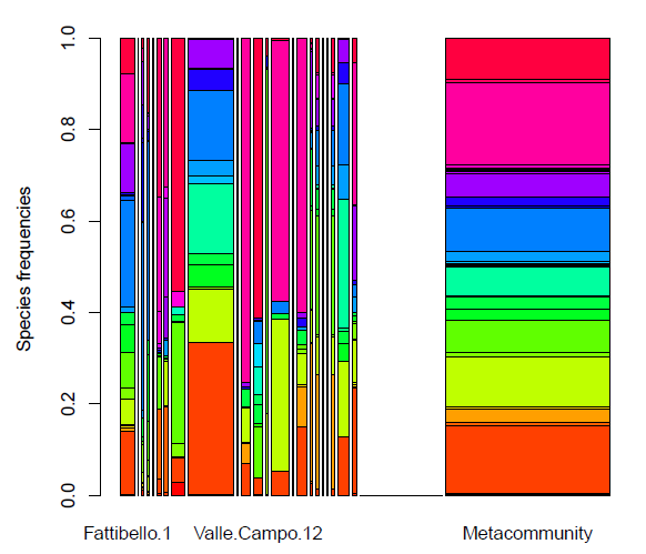
Communities appear to be highly diversified, with several species present in only 2 or 3 stations and some others with high abundance in only one station. Notice that the estimated sample coverage is almost one, i.e. there is no need for bias correction in the estimation of entropy.
> Coverage(Ns=delta.mc1$Ns)
[1] 1
We now compute biodiversity partitioning with order q = 1 and then we analyze the diversity profiles
> delta.part=DivPart(q=1,delta.mc1,Bias=F)
> summary(delta.part)
Diversity partitioning of order 1 of MetaCommunity delta.mc1 with correction:
Best Alpha diversity of communities:
| Fattibello.1 | Fattibello.2 | Fattibello.3 | Fattibello.4 | Goro.scanno.5 |
| 10.084968 | 8.532195 | 7.632217 | 6.109452 | 10.357617 |
| Goro.scanno.6 | Goro.scanno.7 | Smarlacca.8 | Smarlacca.9 | Taglio.della.Falce.10 |
| 5.636836 | 6.068452 | 3.750083 | 7.322140 | 5.337300 |
| Taglio.della.Falce.11 | Valle.Campo.12 | Valle.Campo.13 | Valle.di.Giralda.14 | Valle.di.Gorino.15 |
| 2.622559 | 4.215430 | 2.152055 | 2.773469 | 4.938679 |
| Valle.di.Gorino.16 | Valle.di.Gorino.17 | Valle.di.Gorino.18 | Valle.di.Goro.19 | Valle.di.Goro.20 |
| 3.986790 | 7.025287 | 8.938290 | 6.837332 | 8.422012 |
| Valle.di.Goro.21 | Valle.Magnavacca.22 | Valle.Spavola.23 | ||
| 8.938290 | 7.348205 | 7.155471 | ||
Total alpha diversity of the communities:
[1] 5.527976
Beta diversity of the communities:
[1] 2.524239
Gamma diversity of the metacommunity:
[1] 13.95393
> plot(delta.part,main="q=1")
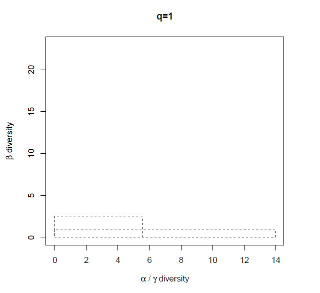
The \(\gamma\) diversity corresponding to the Shannon index (Tsallis entropy of order 1) is about 14 (effective number of species of order 1) out of 47 species, \(\alpha\) diversity is 5.53 showing an average effective number of species at community level of about 6 and \(\beta\) diversity returns 3 effective communities.
> qq=seq(0,2,by=0.1)
> divP.delta=DivProfile(qq,delta.mc1)
> plot(divP.delta)
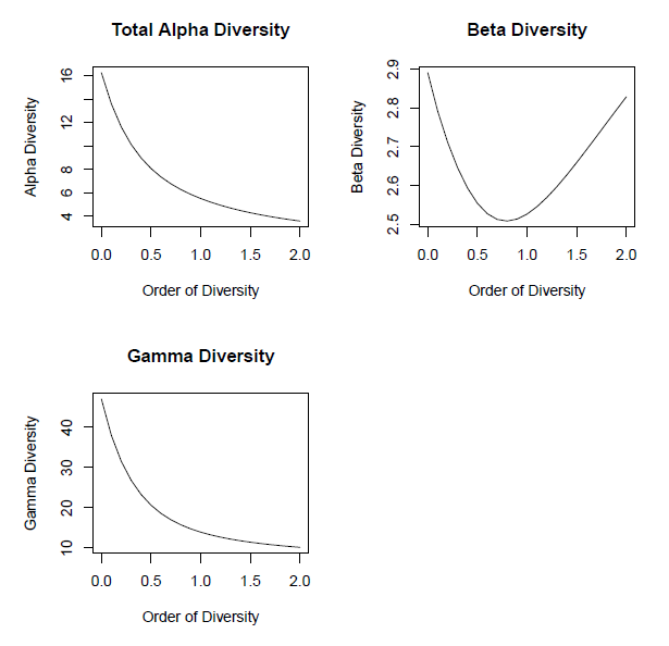
As expected, \(\alpha\) and \(\gamma\) diversity profiles show decreasing values as less importance is given to rare species (increasing index order). \(\beta\) diversity at first decreases reaching a minimum with q = 0:8 and 2.508 effective communities, it increases again up to 2.83 effective communities when q = 2. As an example we compute the simulated confidence intervals for \(\alpha\), \(\beta\) and \(\gamma\) diversity with q = 1:
> divE.delta=DivEst(q=1,MC=delta.mc1,Simulations=100,Biased=FALSE,Correction="Best")
=========================================================
> summary(divE.delta)
Diversity partitioning of order 1 of MetaCommunity MC with correction:
Best Alpha diversity of communities:
| Fattibello.1 | Fattibello.2 | Fattibello.3 | Fattibello.4 | Goro.scanno.5 |
| 10.084968 | 8.532195 | 7.632217 | 6.109452 | 10.357617 |
| Goro.scanno.6 | Goro.scanno.7 | Smarlacca.8 | Smarlacca.9 | Taglio.della.Falce.10 |
| 5.636836 | 6.068452 | 3.750083 | 7.322140 | 5.337300 |
| Taglio.della.Falce.11 | Valle.Campo.12 | Valle.Campo.13 | Valle.di.Giralda.14 | Valle.di.Gorino.15 |
| 2.622559 | 4.215430 | 2.152055 | 2.773469 | 4.938679 |
| Valle.di.Gorino.16 | Valle.di.Gorino.17 | Valle.di.Gorino.18 | Valle.di.Goro.19 | Valle.di.Goro.20 |
| 3.986790 | 7.025287 | 8.938290 | 6.837332 | 8.422012 |
| Valle.di.Goro.21 | Valle.Magnavacca.22 | Valle.Spavola.23 | ||
| 8.938290 | 7.348205 | 7.155471 |
Total alpha diversity of the communities:
[1] 5.527976
Beta diversity of the communities:
[1] 2.524239
Gamma diversity of the metacommunity:
[1] 13.95393
Quantiles of simulations (alpha, beta and gamma diviersity):
| 0% | 10% | 50% | 10% | 25% | 50% | 75% | 90% | 95% | 99% | 100% |
| 5.505946 | 5.518023 | 5.528053 | 5.518023 | 5.523060 | 5.528053 | 5.533624 | 5.538404 | 5.541266 | 5.543972 | 5.546989 |
| 0% | 10% | 50% | 10% | 25% | 50% | 75% | 90% | 95% | 99% | 100% |
| 2.516848 | 2.520032 | 2.524142 | 2.520032 | 2.521520 | 2.524142 | 2.526843 | 2.528266 | 2.529381 | 2.531942 | 2.534291 |
| 0% | 10% | 50% | 10% | 25% | 50% | 75% | 90% | 95% | 99% | 100% |
| 13.91246 | 13.93033 | 13.95376 | 13.93033 | 13.94107 | 13.95376 | 13.96433 | 13.97925 | 13.98359 | 13.99438 | 14.00518 |
> plot(divE.delta)
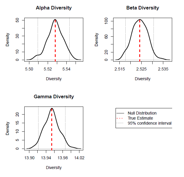
Simulations show very little variability in the estimated values. We now analyze biodiversity with communities defined at the lagoon spatial scale. We modify the definition of the meta-community by taking the the average abundance in each lagoon. The number of available lagoons can be obtained from the column of lagoons labels in the env dataframe. The function levels isolates the different categories in a factor, the number of categories is what we need and we obtain it using the function length
> nl=length(levels(env$Lagoon))
> delta.lag=data.frame(matrix(0,nrow(delta),nl))
> row.names(delta.lag)=row.names(delta)
> colnames(delta.lag)=levels(env$Lagoon)
> #### to aggregate by lagoon we apply the mean to each row of the delta dataset
> for( i in 1:nrow(delta)){<br> + delta.lag[i,]=tapply(t(delta[i,]),env$Lagoon,mean)<br> + }
We create the meta-community
> delta.lag.mc=MetaCommunity(delta.lag,apply(delta.lag,2,sum))
Notice that there's one lagoon where one species is largely more abundant than the others
> plot(delta.lag.mc,col=colorRampPalette(c("red","green","blue"))(47))
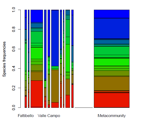
To see which species is responsible for the warning we write:
> sort(round(apply(delta.lag,1,sum)/sum(apply(delta.lag,1,sum)),5))
| Bittium.reticulatum | Lentidium.mediterraneum | Tellina.sp. | Crassostrea.sp. |
| 0.00000 | 0.00000 | 0.00000 | 0.00002 |
| Ensis.siliqua. | Carcinus.aestuarii | Ascidiacei.spp. | Lekanesphaera.hookeri |
| 0.00005 | 0.00011 | 0.00016 | 0.00016 |
| Nassarius.reticulatus. | Anadara.inaequivalvis | Palaemon.elegans | Mytilus.galloprovincialis |
| 0.00017 | 0.00026 | 0.00031 | 0.00038 |
| Mytilaster.minimus | Ostrea.edulis | Brachynotus.sexdentatus | Ruditapes.philippinarum |
| 0.00041 | 0.00041 | 0.00048 | 0.00052 |
| Phyllodoce.lineata. | Cyclope.neritea | Actiniari.spp. | Heteromastus.filiformis. |
| 0.00060 | 0.00066 | 0.00074 | 0.00088 |
| Ruditapes.decussatus | Haminoea.hydatis | Nephtys.hombergii | Balanidae.spp. |
| 0.00117 | 0.00127 | 0.00147 | 0.00167 |
| Abra.segmentum | Littorina.littorea | Spio.decoratus. | Sphaeroma.serratum |
| 0.00227 | 0.00234 | 0.00342 | 0.00363 |
| Prionospio.multibranchiata | Idotea.balthica | Ampelisca.sp. | Lucifer.typus |
| 0.00380 | 0.00433 | 0.00466 | 0.00477 |
| Turbellaria | Cerastoderma.glaucum | Arcuatula.senhousia | Oligochaeta.spp. |
| 0.00478 | 0.00831 | 0.01673 | 0.02038 |
| Ficopomatus.enigmaticus | Microdeutopus.gryllotalpa | Gammarus.aequicauda. | Polydora.ciliata |
| 0.02169 | 0.02344 | 0.02490 | 0.04470 |
| Chironomus.salinarius | Hydroides.dianthus | Ventrosia.ventrosa | Monocorophium.insidiosum |
| 0.05222 | 0.07469 | 0.08177 | 0.08757 |
| Capitella.capitata | Alitta.succinea | Streblospio.shrubsolii | |
| 0.14226 | 0.14812 | 0.20732 |
and we can see that Streblospio shrubsolii is the most abundant species in the meta-community. Now by writing:
> sort(apply(delta.lag,2,sum))
| Valle di Goro | Goro scanno | Valle di Gorino | Fattibello | Valle Spavola | Taglio della Falce |
| 5209.221 | 8153.791 | 11261.864 | 12598.863 | 13158.650 | 13922.968 |
| Valle Campo | Valle Magnavacca | Valle di Giralda | Smarlacca | ||
| 14526.201 | 29398.435 | 48605.790 | 80404.341 |
we can see that Valle di Giralda and Smarlacca are the two lagoons with the most abundant portion of individuals. To have some further insight in the communities structure we draw a bar plot of the communities
> barplot(as.matrix(delta.lag),col=colorRampPalette(c("red","green","blue"))(47),cex.names=0.5)
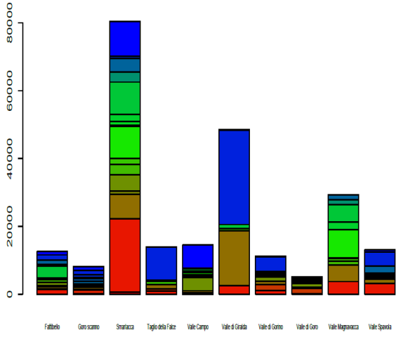
From the bar plot it is clear that both Smarlacca and Valle di Giralda have a dominant species, by looking directly at the abundances we see that the Alitta succinea[1] is the most abundant species at Smarlacca while Streblospio shrubsolii[2] is the most abundant in Valle di Giralda. In this two lagoons the probability of an individual to belong to this two species is obtained by dividing the amount of each species in each lagoon by the total abundance of individuals of the species in the same lagoon:
> delta.lag[c(3,44),c(3,6)]/c(sum(delta.lag[,3]),sum(delta.lag[,6]))
| Smarlacca | Valle di Giralda | |
| Alitta.succinea | 0.268859892 | 0.03168697 |
| Streblospio.shrubsolii | 0.001302983 | 0.57221899 |
From this simple computation we can clearly see that Streblospio shrubsolii in the Valle di Giralda lagoon is responsible for the warning. The biodiversity partitioning is obtained:
> divP.delta.lag=DivPart(q=1,delta.lag.mc)
> summary(divP.delta.lag)
Diversity partitioning of order 1 of MetaCommunity delta.lag.mc Alpha diversity of communities:
| Fattibello | Goro scanno | Smarlacca | Taglio della Falce | Valle Campo | Valle di Giralda |
| 10.741547 | 12.542096 | 10.049474 | 3.104848 | 4.996149 | 2.773469 |
| Valle di Gorino | Valle di Goro | Valle Magnavacca | Valle Spavola | ||
| 7.852548 | 9.918649 | 7.346912 | 7.144584 |
Total alpha diversity of the communities: [1] 6.510694 Beta diversity of the communities: [1] 1.900928 Gamma diversity of the metacommunity: [1] 12.37636
and the profiles:
> divP.delta.lag=DivProfile(qq,delta.lag.mc)
> plot(divP.delta.lag)
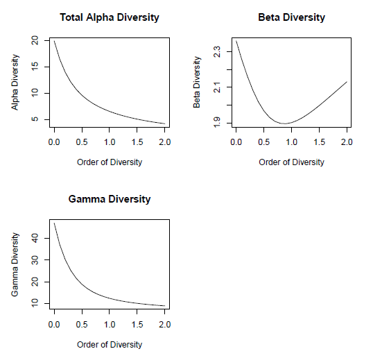
The same behavior seen before is shown. Then we aggregate further and compute biodiversity profiles with communities defined at the system spatial scale. We adopt the same procedure seen for the lagoons, this time we use the System column in the env data.frame
> ns=length(levels(env$System))
> ### define a new object
> delta.sys=data.frame(matrix(0,nrow(delta),ns))
> row.names(delta.sys)=row.names(delta)
> colnames(delta.sys)=levels(env$System)
> #### to aggregate by lagoon we apply to each row of the delta dataset the mean
> for( i in 1:nrow(delta)){<br> + delta.sys[i,]=tapply(t(delta[i,]),env$System,mean)<br> + }
and we create the metacommunity
> delta.sys.mc=MetaCommunity(delta.sys,apply(delta.sys,2,sum))
> plot(delta.sys.mc,col=colorRampPalette(c("red","green","blue"))(47))
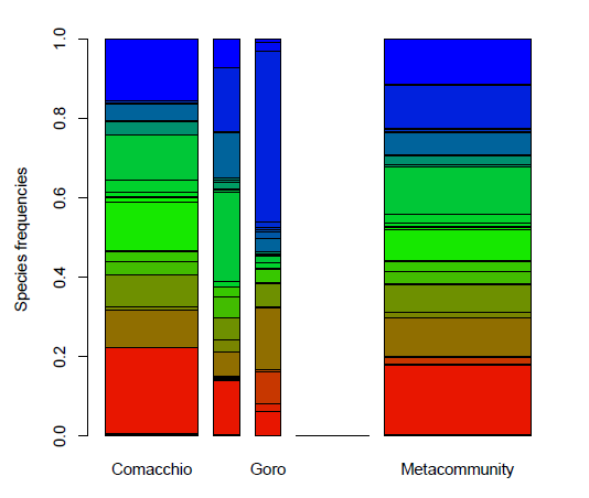
Differences have been considerably smoothed. Now we can partition diversity with communities defined by systems
> divP.delta.sys=DivPart(q=1,delta.sys.mc)
> summary(divP.delta.sys)
Diversity partitioning of order 1 of MetaCommunity delta.sys.mc Alpha diversity of communities:
| Comacchio | Fattibello | Goro |
| 10.734190 | 10.808570 | 8.188278 |
Total alpha diversity of the communities:
[1] 10.2362
Beta diversity of the communities:
[1] 1.34688
Gamma diversity of the metacommunity:
[1] 13.78694
and compute profiles
> divP.delta.sys=DivProfile(qq,delta.sys.mc)
> plot(divP.delta.sys)
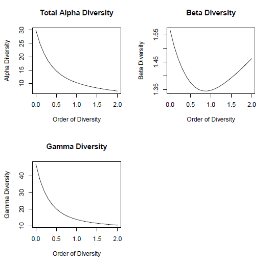
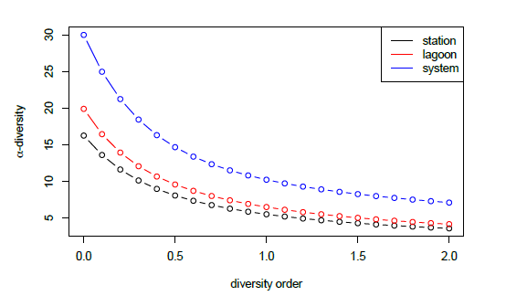
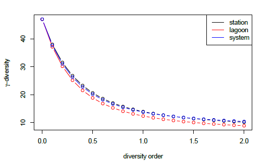
No changes in the general behavior of profiles, to compare them:
> plot(qq,divP.delta$TotalAlphaDiversity,type="b",
+ ylab=expression(paste(alpha,"-diversity",sep="")),xlab="diversity order",
+ ylim=range(c(divP.delta$TotalAlphaDiversity,divP.delta.lag$TotalAlphaDiversity,divP.
+ delta.sys$TotalAlphaDiversity)))
> lines(qq,divP.delta.lag$TotalAlphaDiversity,type="b",col=2)
> lines(qq,divP.delta.sys$TotalAlphaDiversity,type="b",col=4)
> legend("topright",c("station","lagoon","system"),lty=1,col=c(1,2,4))
> plot(qq,divP.delta$GammaDiversity,type="b",
+ ylab=expression(paste(gamma,"-diversity",sep="")),xlab="diversity order",
+ ylim=range(c(divP.delta$GammaDiversity,divP.delta.lag$GammaDiversity,
+ divP.delta.sys$GammaDiversity)))
> lines(qq,divP.delta.lag$GammaDiversity,type="b",col=2)
> lines(qq,divP.delta.sys$GammaDiversity,type="b",col=4)
> legend("topright",c("station","lagoon","system"),lty=1,col=c(1,2,4))
> plot(qq,divP.delta$TotalBetaDiversity,type="b",
+ ylab=expression(paste(beta,"-diversity",sep="")),xlab="diversity order",
+ ylim=range(c(1,divP.delta$TotalBetaDiversity,divP.delta.lag$TotalBetaDiversity,
+ divP.delta.sys$TotalBetaDiversity)))
> lines(qq,divP.delta.lag$TotalBetaDiversity,type="b",col=2)
> lines(qq,divP.delta.sys$TotalBetaDiversity,type="b",col=4)
> legend("top",c("station","lagoon","system"),lty=1,col=c(1,2,4),cex=0.5)
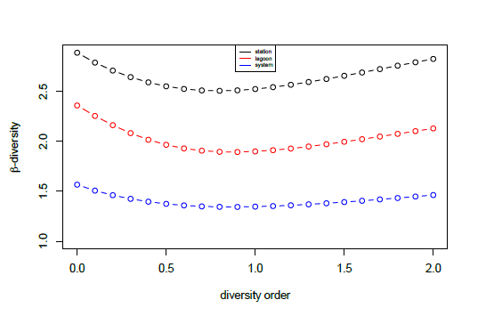
As expected there is a considerable change in the values of alpha and beta diversity when changing the definition of community (spatial scale).
Partizione della biodiversitá dei dati del delta del fiume Po
In questa sezione si svilupperá una prima parte del case study del delta del fiume Po. Il set di dati é stato raccolto da 23 stazioni di monitoraggio raggruppato in 10 lagune divisi in 3 sistemi di lagune (Goro, Fattibello e Comacchio) nel delta del fiume po (Mare Adriatico Settentrionale). Piú specificatamente i dati riguardano i macroinvertebrati bentici raccolti dalle stazioni di monitoraggio presentando da uno a tre tipi di habitat dominanti, definiti da una classificazione fattoriale della granulometria del sedimento (sabbia, fango) e la copertura/tipo vegetativo (senza vegetazione, macrofiti sommersi, macrofiti emersi e macroalge) come in Basset et al. (2008b). In ogni laguna, sono state effettuate campagne di campionamento con da una a tre stazioni di monitoraggio per tipo di habitat. In questo caso si considera una gerarchia di scale spaziali multiple, con le stazioni annidate nelle lagune annidate, a loro volta, nei sistemi. Si vuole verificare come la biodiversitá cambia su scale spaziali differenti e con l'ordine della diversitá dando importanza decrescente alle specie rare.
Figure 1: The Po River Delta area
Inanzitutto é necessario leggere i dati da file csv. In due files sono disponibili una tabella faunistica con le densitá degli esemplari come misura di abbondanza e la matrice ambientale:
> delta=read.table("delta1.csv",header=T,sep=";",row.names=1)
> env=read.table("env1.csv",header=T,sep=";",row.names=1)
> str(delta)
'data.frame': 47 obs. of 23 variables:
$ Fattibello.1 : num 1.05 98.52 5409.41 0 24.31 ...
$ Fattibello.2 : num 0 9.72 105.58 0 5.09 ...
$ Fattibello.3 : num 0 57.9 0 0 3.7 ...
$ Fattibello.4 : num 0 2.78 2.32 0 0 ...
$ Goro.scanno.5 : num 2.32 0 152.35 50.01 7.41 ...
$ Goro.scanno.6 : num 0 49.1 294.5 1477.1 0 ...
$ Goro.scanno.7 : num 0 0 66.7 1784.2 0 ...
$ Smarlacca.8 : num 1077 0 1930 0 0 ...
$ Smarlacca.9 : num 0 103 41305 0 0 ...
$ Taglio.della.Falce.10: num 0 0.694 50.694 0 0 ...
$ Taglio.della.Falce.11: num 0 0 1812 0 0 ...
$ Valle.Campo.12 : num 0 38.6 795.2 0 0 ...
$ Valle.Campo.13 : num 0 0 6.03 0 0 ...
$ Valle.di.Giralda.14 : num 0 0 2548 0 0 ...
$ Valle.di.Gorino.15 : num 0 0 29.17 2.78 0 ...
$ Valle.di.Gorino.16 : num 0 0 4260 0 0 ...
$ Valle.di.Gorino.17 : num 0 1.85 163 0 26.86 ...
$ Valle.di.Gorino.18 : num 0 0 107.43 0 8.34 ...
$ Valle.di.Goro.19 : num 0 2.32 308.86 0 6.48 ...
$ Valle.di.Goro.20 : num 0 5.09 0 0 43.99 ...
$ Valle.di.Goro.21 : num 0 0 107.43 0 8.34 ...
$ Valle.Magnavacca.22 : num 0 0 3751 0 0 ...
$ Valle.Spavola.23 : num 0 42.1 3063.1 0 22.7 ...
> str(env)
'data.frame': 23 obs. of 5 variables:
$ System : Factor w/ 3 levels "Comacchio","Fattibello",..: 2 2 2 2 3 3 3 1 1 3 ...
$ Lagoon : Factor w/ 10 levels "Fattibello","Goro scanno",..: 1 1 1 1 2 2 2 3 3 4 ...
$ Vegetation: Factor w/ 4 levels "emacroph","macroa",..: 2 3 3 3 3 3 3 4 4 1 ...
$ Sediment : Factor w/ 2 levels "mud","sand": 1 1 1 1 2 2 2 1 1 1 ...
$ Station : int 1 2 3 4 5 6 7 8 9 10 ...
Ora si procede alla realizzazione di una meta-comunitá definita su scala spaziale locale, ossia a livello di stazione di monitoraggio.
> require(entropart)
É siano i pesi proporzionali all'abbondanza in ogni sito
> delta.mc1=MetaCommunity(delta,apply(delta,2,sum))
> summary(delta.mc1)
Meta-community (class 'MetaCommunity') made of 444401.8 individuals in 23 communities and 47 species.
Its sample coverage is 1
Community weights are:
| Fattibello.1 | Fattibello.2 | Fattibello.3 | Fattibello.4 | Goro.scanno.5 |
| 0.088027504 | 0.003114463 | 0.012038978 | 0.010219690 | 0.011794114 |
| Goro.scanno.6 | Goro.scanno.7 | Smarlacca.8 | Smarlacca.9 | Taglio.della.Falce.10 |
| 0.021810619 | 0.021438634 | 0.082843290 | 0.279010936 | 0.004723890 |
| Taglio.della.Falce.11 | Valle.Campo.12 | Valle.Campo.13 | Valle.di.Giralda.14 | Valle.di.Gorino.15 |
| 0.057935475 | 0.049738592 | 0.015635579 | 0.109373513 | 0.004734829 |
| Valle.di.Gorino.16 | Valle.di.Gorino.17 | Valle.di.Gorino.18 | Valle.di.Goro.19 | Valle.di.Goro.20 |
| 0.063795908 | 0.014026024 | 0.018809731 | 0.007981528 | 0.008374352 |
| Valle.di.Goro.21 | Valle.Magnavacca.22 | Valle.Spavola.23 | ||
| 0.018809731 | 0.066152821 | 0.029609801 |
Community sample numbers of individuals are:
| Fattibello.1 | Fattibello.2 | Fattibello.3 | Fattibello.4 | Goro.scanno.5 |
| 39119.584 | 1384.073 | 5350.144 | 4541.649 | 5241.326 |
| Goro.scanno.6 | Goro.scanno.7 | Smarlacca.8 | Smarlacca.9 | Taglio.della.Falce.10 |
| 9692.679 | 9527.368 | 36815.710 | 123992.972 | 2099.306 |
| Taglio.della.Falce.11 | Valle.Campo.12 | Valle.Campo.13 | Valle.di.Giralda.14 | Valle.di.Gorino.15 |
| 25746.631 | 22103.922 | 6948.480 | 48605.790 | 2104.167 |
| Valle.di.Gorino.16 | Valle.di.Gorino.17 | Valle.di.Gorino.18 | Valle.di.Goro.19 | Valle.di.Goro.20 |
| 28351.018 | 6233.191 | 8359.079 | 3547.006 | 3721.577 |
| Valle.di.Goro.21 | Valle.Magnavacca.22 | Valle.Spavola.23 | ||
| 8359.079 | 29398.435 | 13158.650 |
Community sample coverages are:
| Fattibello.1 | Fattibello.2 | Fattibello.3 | Fattibello.4 | Goro.scanno.5 |
| 0.9999233 | 1.0000000 | 0.9998127 | 0.9997796 | 0.9996175 |
| Goro.scanno.6 | Goro.scanno.7 | Smarlacca.8 | Smarlacca.9 | Taglio.della.Falce.10 |
| 0.9998968 | 0.9996847 | 1.0000000 | 1.0000000 | 1.0000000 |
| Taglio.della.Falce.11 | Valle.Campo.12 | Valle.Campo.13 | Valle.di.Giralda.14 | Valle.di.Gorino.15 |
| 1.0000000 | 1.0000000 | 1.0000000 | 1.0000000 | 1.0000000 |
| Valle.di.Gorino.16 | Valle.di.Gorino.17 | Valle.di.Gorino.18 | Valle.di.Goro.19 | Valle.di.Goro.20 |
| 1.0000000 | 0.9996785 | 0.9998802 | 0.9997176 | 0.9994603 |
| Valle.di.Goro.21 | Valle.Magnavacca.22 | Valle.Spavola.23 | ||
| 0.9998802 | 1.0000000 | 0.9998479 |
Si ottiene la rappresentazione grafica della meta-comunitá
> plot(delta.mc1,col=rainbow(48))
Le comunitá sembrano altamente diversificati, con molte specie presenti in solo 2 o 3 stazioni ed alcune altre con grossa abbondanza in una stazione sola. Si noti che la copertura campionaria é pressocché uno, ossia non vi é la necessitá per la correzione del bias per la stima dell'entropia.
> Coverage(Ns=delta.mc1$Ns)
[1] 1
ora si puó calcolare la partizione della biodiversitá di ordine q=1 e si nanalizzano i profili di diversitá
> delta.part=DivPart(q=1,delta.mc1,Bias=F)
> summary(delta.part)
Diversity partitioning of order 1 of MetaCommunity delta.mc1 with correction:
Best Alpha diversity of communities:
| Fattibello.1 | Fattibello.2 | Fattibello.3 | Fattibello.4 | Goro.scanno.5 |
| 10.084968 | 8.532195 | 7.632217 | 6.109452 | 10.357617 |
| Goro.scanno.6 | Goro.scanno.7 | Smarlacca.8 | Smarlacca.9 | Taglio.della.Falce.10 |
| 5.636836 | 6.068452 | 3.750083 | 7.322140 | 5.337300 |
| Taglio.della.Falce.11 | Valle.Campo.12 | Valle.Campo.13 | Valle.di.Giralda.14 | Valle.di.Gorino.15 |
| 2.622559 | 4.215430 | 2.152055 | 2.773469 | 4.938679 |
| Valle.di.Gorino.16 | Valle.di.Gorino.17 | Valle.di.Gorino.18 | Valle.di.Goro.19 | Valle.di.Goro.20 |
| 3.986790 | 7.025287 | 8.938290 | 6.837332 | 8.422012 |
| Valle.di.Goro.21 | Valle.Magnavacca.22 | Valle.Spavola.23 | ||
| 8.938290 | 7.348205 | 7.155471 | ||
Total alpha diversity of the communities:
[1] 5.527976
Beta diversity of the communities:
[1] 2.524239
Gamma diversity of the metacommunity:
[1] 13.95393
> plot(delta.part,main="q=1")
La diversitá \(\gamma\) corrispondente all'indice di Shannon (entropia di Tsallis di ordine 1) é circa 14 (numero effettivo di specie di ordine 1) su un totale di 47 specie, la diversitá \(\alpha\) é 5.53 indicando un numero medio di specie a livello di comunitá di circa 6 la diversiá \(\beta\) restituisce 3 comunitá effettive.
> qq=seq(0,2,by=0.1)
> divP.delta=DivProfile(qq,delta.mc1)
> plot(divP.delta)
Come previsto, i profili delle diversitá \(\alpha\) e \(\gamma\) mostrano valori decrescenti siccome é data meno importanza alle specie rare (ordine di indice crescente). La diversitá \(\beta\) inizialmente decresce raggiungendo un minimo con q = 0.8 e 2.508 comunitá effettive, successivamente cresce fino a 2.83 comunitá effettive quando q=2. Come esempio si possono calcolare gli intervalli di confidenza simulati per le diversitá \(\alpha\), \(\beta\) and \(\gamma\) con q = 1:
> divE.delta=DivEst(q=1,MC=delta.mc1,Simulations=100,Biased=FALSE,Correction="Best")
=========================================================
> summary(divE.delta)
Diversity partitioning of order 1 of MetaCommunity MC with correction:
Best Alpha diversity of communities:
| Fattibello.1 | Fattibello.2 | Fattibello.3 | Fattibello.4 | Goro.scanno.5 |
| 10.084968 | 8.532195 | 7.632217 | 6.109452 | 10.357617 |
| Goro.scanno.6 | Goro.scanno.7 | Smarlacca.8 | Smarlacca.9 | Taglio.della.Falce.10 |
| 5.636836 | 6.068452 | 3.750083 | 7.322140 | 5.337300 |
| Taglio.della.Falce.11 | Valle.Campo.12 | Valle.Campo.13 | Valle.di.Giralda.14 | Valle.di.Gorino.15 |
| 2.622559 | 4.215430 | 2.152055 | 2.773469 | 4.938679 |
| Valle.di.Gorino.16 | Valle.di.Gorino.17 | Valle.di.Gorino.18 | Valle.di.Goro.19 | Valle.di.Goro.20 |
| 3.986790 | 7.025287 | 8.938290 | 6.837332 | 8.422012 |
| Valle.di.Goro.21 | Valle.Magnavacca.22 | Valle.Spavola.23 | ||
| 8.938290 | 7.348205 | 7.155471 |
Total alpha diversity of the communities:
[1] 5.527976
Beta diversity of the communities:
[1] 2.524239
Gamma diversity of the metacommunity:
[1] 13.95393
Quantiles of simulations (alpha, beta and gamma diviersity):
| 0% | 10% | 50% | 10% | 25% | 50% | 75% | 90% | 95% | 99% | 100% |
| 5.505946 | 5.518023 | 5.528053 | 5.518023 | 5.523060 | 5.528053 | 5.533624 | 5.538404 | 5.541266 | 5.543972 | 5.546989 |
| 0% | 10% | 50% | 10% | 25% | 50% | 75% | 90% | 95% | 99% | 100% |
| 2.516848 | 2.520032 | 2.524142 | 2.520032 | 2.521520 | 2.524142 | 2.526843 | 2.528266 | 2.529381 | 2.531942 | 2.534291 |
| 0% | 10% | 50% | 10% | 25% | 50% | 75% | 90% | 95% | 99% | 100% |
| 13.91246 | 13.93033 | 13.95376 | 13.93033 | 13.94107 | 13.95376 | 13.96433 | 13.97925 | 13.98359 | 13.99438 | 14.00518 |
> plot(divE.delta)
Le simulazioni mostrano variabilitá molto piccole dei valori stimati. Ora si procede all'anilisi della biodiversitá con comunitá definite su scala spaziale a livello di laguna. Si modifica la definizione di meta-comunitá prendendo l'abbondanza media di ogni laguna. Il numero delle lagune disponibili puó essere ottenuto dalla colonna delle etichette delle lagune nel dataframe env. La funzione levels isola le categorie differenti in un fattore, il numero di categorie che serve per proseguire l'analisi viene ottenuto utilizzando la funzione length
> nl=length(levels(env$Lagoon))
> delta.lag=data.frame(matrix(0,nrow(delta),nl))
> row.names(delta.lag)=row.names(delta)
> colnames(delta.lag)=levels(env$Lagoon)
> #### to aggregate by lagoon we apply the mean to each row of the delta dataset
> for( i in 1:nrow(delta)){<br> + delta.lag[i,]=tapply(t(delta[i,]),env$Lagoon,mean)<br> + }
Si crea la meta-comunitá
> delta.lag.mc=MetaCommunity(delta.lag,apply(delta.lag,2,sum))
Si noti che esiste una laguna dove una specie é largamente piú abbondante di altre
> plot(delta.lag.mc,col=colorRampPalette(c("red","green","blue"))(47))
Per vedere quale specie é responsabile per l'avvertimento (warning) si digita:
> sort(round(apply(delta.lag,1,sum)/sum(apply(delta.lag,1,sum)),5))
| Bittium.reticulatum | Lentidium.mediterraneum | Tellina.sp. | Crassostrea.sp. |
| 0.00000 | 0.00000 | 0.00000 | 0.00002 |
| Ensis.siliqua. | Carcinus.aestuarii | Ascidiacei.spp. | Lekanesphaera.hookeri |
| 0.00005 | 0.00011 | 0.00016 | 0.00016 |
| Nassarius.reticulatus. | Anadara.inaequivalvis | Palaemon.elegans | Mytilus.galloprovincialis |
| 0.00017 | 0.00026 | 0.00031 | 0.00038 |
| Mytilaster.minimus | Ostrea.edulis | Brachynotus.sexdentatus | Ruditapes.philippinarum |
| 0.00041 | 0.00041 | 0.00048 | 0.00052 |
| Phyllodoce.lineata. | Cyclope.neritea | Actiniari.spp. | Heteromastus.filiformis. |
| 0.00060 | 0.00066 | 0.00074 | 0.00088 |
| Ruditapes.decussatus | Haminoea.hydatis | Nephtys.hombergii | Balanidae.spp. |
| 0.00117 | 0.00127 | 0.00147 | 0.00167 |
| Abra.segmentum | Littorina.littorea | Spio.decoratus. | Sphaeroma.serratum |
| 0.00227 | 0.00234 | 0.00342 | 0.00363 |
| Prionospio.multibranchiata | Idotea.balthica | Ampelisca.sp. | Lucifer.typus |
| 0.00380 | 0.00433 | 0.00466 | 0.00477 |
| Turbellaria | Cerastoderma.glaucum | Arcuatula.senhousia | Oligochaeta.spp. |
| 0.00478 | 0.00831 | 0.01673 | 0.02038 |
| Ficopomatus.enigmaticus | Microdeutopus.gryllotalpa | Gammarus.aequicauda. | Polydora.ciliata |
| 0.02169 | 0.02344 | 0.02490 | 0.04470 |
| Chironomus.salinarius | Hydroides.dianthus | Ventrosia.ventrosa | Monocorophium.insidiosum |
| 0.05222 | 0.07469 | 0.08177 | 0.08757 |
| Capitella.capitata | Alitta.succinea | Streblospio.shrubsolii | |
| 0.14226 | 0.14812 | 0.20732 |
e si vede che lo Streblospio shrubsolii é la specie piú abbondante nella meta-comunitá. Now by writing:
> sort(apply(delta.lag,2,sum))
| Valle di Goro | Goro scanno | Valle di Gorino | Fattibello | Valle Spavola | Taglio della Falce |
| 5209.221 | 8153.791 | 11261.864 | 12598.863 | 13158.650 | 13922.968 |
| Valle Campo | Valle Magnavacca | Valle di Giralda | Smarlacca | ||
| 14526.201 | 29398.435 | 48605.790 | 80404.341 |
si vede che Valle di Giralda e Smarlacca sono le due lagune con la porzione piú abbondante di esemplari. Per approfondire ulteriormente la struttura delle comunitá si disegna un grafico a barre delle comunitá
> barplot(as.matrix(delta.lag),col=colorRampPalette(c("red","green","blue"))(47),cex.names=0.5)
Dal grafico é evidente che Smarlacca e VAlle di Giralda hanno una specie dominante, guardando le abbondanze si vede che l'Alitta succinea[1] è la specie piú abbondante a Smarlacca mentre lo Streblospio shrubsolii[2] è il piú abbondante in Valle di Giralda. In queste due lagune, la probabilitá di un esemplare di appartenere a queste due specie è ottenuto dividendo la quantitá di ogni specie in ogni laguna per la totale abbondanza di esemplari della specie nella stessa laguna:
> delta.lag[c(3,44),c(3,6)]/c(sum(delta.lag[,3]),sum(delta.lag[,6]))
| Smarlacca | Valle di Giralda | |
| Alitta.succinea | 0.268859892 | 0.03168697 |
| Streblospio.shrubsolii | 0.001302983 | 0.57221899 |
Da questo semplice calcolo si vede chiaramente che lo Streblospio shrubsolii nella laguna di Valle di Giralda é il responsabile del precedente avvertimento (warning). La partizione della biodiversitá si ottiene:
> divP.delta.lag=DivPart(q=1,delta.lag.mc)
> summary(divP.delta.lag)
Diversity partitioning of order 1 of MetaCommunity delta.lag.mc Alpha diversity of communities:
| Fattibello | Goro scanno | Smarlacca | Taglio della Falce | Valle Campo | Valle di Giralda |
| 10.741547 | 12.542096 | 10.049474 | 3.104848 | 4.996149 | 2.773469 |
| Valle di Gorino | Valle di Goro | Valle Magnavacca | Valle Spavola | ||
| 7.852548 | 9.918649 | 7.346912 | 7.144584 |
Total alpha diversity of the communities: [1] 6.510694 Beta diversity of the communities: [1] 1.900928 Gamma diversity of the metacommunity: [1] 12.37636
e i profili:
> divP.delta.lag=DivProfile(qq,delta.lag.mc)
> plot(divP.delta.lag)
Si vedo lo stesso andamento di quello precedente. Quindi si aggrega ulteriormente e si calcolano i profili di biodiversitá con le comunitá su scala spaziale del sistema. Si adotta la stessa procedura vista per le lagune, solo che si utilizzerá la colonna System nel data.frame env
> ns=length(levels(env$System))
> ### define a new object
> delta.sys=data.frame(matrix(0,nrow(delta),ns))
> row.names(delta.sys)=row.names(delta)
> colnames(delta.sys)=levels(env$System)
> #### to aggregate by lagoon we apply to each row of the delta dataset the mean
> for( i in 1:nrow(delta)){<br> + delta.sys[i,]=tapply(t(delta[i,]),env$System,mean)<br> + }
e si crea la meta-comunitá
> delta.sys.mc=MetaCommunity(delta.sys,apply(delta.sys,2,sum))
> plot(delta.sys.mc,col=colorRampPalette(c("red","green","blue"))(47))
Le differenze sono state considerevolmente attenuate. Ora si puó partizionare la diversitá con le comunitá definite da Systems
> divP.delta.sys=DivPart(q=1,delta.sys.mc)
> summary(divP.delta.sys)
Diversity partitioning of order 1 of MetaCommunity delta.sys.mc Alpha diversity of communities:
| Comacchio | Fattibello | Goro |
| 10.734190 | 10.808570 | 8.188278 |
Total alpha diversity of the communities:
[1] 10.2362
Beta diversity of the communities:
[1] 1.34688
Gamma diversity of the metacommunity:
[1] 13.78694
e si calcolano i profili
> divP.delta.sys=DivProfile(qq,delta.sys.mc)
> plot(divP.delta.sys)
Nessune variazioni nel comportamento generale dei profili, per confrontarli:
> plot(qq,divP.delta$TotalAlphaDiversity,type="b",
+ ylab=expression(paste(alpha,"-diversity",sep="")),xlab="diversity order",
+ ylim=range(c(divP.delta$TotalAlphaDiversity,divP.delta.lag$TotalAlphaDiversity,divP.
+ delta.sys$TotalAlphaDiversity)))
> lines(qq,divP.delta.lag$TotalAlphaDiversity,type="b",col=2)
> lines(qq,divP.delta.sys$TotalAlphaDiversity,type="b",col=4)
> legend("topright",c("station","lagoon","system"),lty=1,col=c(1,2,4))
> plot(qq,divP.delta$GammaDiversity,type="b",
+ ylab=expression(paste(gamma,"-diversity",sep="")),xlab="diversity order",
+ ylim=range(c(divP.delta$GammaDiversity,divP.delta.lag$GammaDiversity,
+ divP.delta.sys$GammaDiversity)))
> lines(qq,divP.delta.lag$GammaDiversity,type="b",col=2)
> lines(qq,divP.delta.sys$GammaDiversity,type="b",col=4)
> legend("topright",c("station","lagoon","system"),lty=1,col=c(1,2,4))
> plot(qq,divP.delta$TotalBetaDiversity,type="b",
+ ylab=expression(paste(beta,"-diversity",sep="")),xlab="diversity order",
+ ylim=range(c(1,divP.delta$TotalBetaDiversity,divP.delta.lag$TotalBetaDiversity,
+ divP.delta.sys$TotalBetaDiversity)))
> lines(qq,divP.delta.lag$TotalBetaDiversity,type="b",col=2)
> lines(qq,divP.delta.sys$TotalBetaDiversity,type="b",col=4)
> legend("top",c("station","lagoon","system"),lty=1,col=c(1,2,4),cex=0.5)
Come previsto vi sono delle variazioni considerevoli nei valori della diversitá alfa e beta quando la cambia la definizione della comunitá (scala spaziale).
The Po River Delta: Mixed effects models
We are interested in assessing which spatial scale (system, lagoon or monitoring station) seems more relevant in terms of representation of biodiversity variation. The fixed effects are given by the factors Vegetation and Sediment that describe the station environment. Being both explanatory variables categorical, their inclusion in the fixed part of the model implies that a fixed intercept for each combination of categories is estimated, plus the nested random effects of the the System and Lagoon factors. For comparison, we first consider a model with no explanatory variables, including only one fixed intercept and random intercepts ruled by the nested effects of System and Lagoon. Nested effects are represented using the syntax effect1/effect2/effect3....
> require(nlme)
> alpha.1=delta.part$CommunityAlphaEntropies
> sys=env$System
> lag=env$Lagoon
> mod0.delta=lme(alpha.1~1,random=~1|sys/lag,data=env,method="ML")
> summary(mod0.delta)
Linear mixed-effects model fit by maximum likelihood
Data: env
| AIC | BIC | logLik |
| 32.47187 | 37.01384 | -12.23593 |
Random effects:
Formula: ~1 | sys
(Intercept)
StdDev: 7.931876e-06
Formula: ~1 | lag %in% sys
(Intercept) Residual
StdDev: 0.2696757 0.3427638
Fixed effects: alpha.1 ~ 1
| Value | Std.Error | DF | t-value | p-value | |
| (Intercept) | 1.723163 | 0.1172432 | 13 | 14.69735 | 0 |
Standardized Within-Group Residuals:
| Min | Q1 | Med | Q3 | Max |
| -1.7897264 | -0.4813381 | 0.1724562 | 0.5263777 | 1.3500645 |
Number of Observations: 23
Number of Groups:
| sys | lag | %in% | sys |
| 3 | 10 |
We estimate the model including both explanatory variables: Vegetation and Sediment
> mod1.delta=lme(alpha.1~Vegetation+Sediment,random=~1|sys/lag,data=env,method="ML")
> summary(mod1.delta)
Linear mixed-effects model fit by maximum likelihood
Data: env
| AIC | BIC | logLik |
| 27.68141 | 36.76536 | -5.840703 |
Random effects: Formula: ~1 | sys
| (Intercept) | |
| StdDev: | 5.495947e-06 |
Formula: ~1 | lag %in% sys
| (Intercept) | Residual | |
| StdDev: | 1.127679e-06 | 0.3119242 |
Fixed effects: alpha.1 ~ Vegetation + Sediment
| Value | Std.Error | DF | t-value | p-value | |
| Intercept) | 1.4047387 | 0.1762978 | 11 | 7.967989 | 0.0000 |
| Vegetationmacroa | 0.7110108 | 0.2275994 | 11 | 3.123957 | 0.0097 |
| Vegetationnone | 0.4233437 | 0.2275994 | 11 | 1.860039 | 0.0898 |
| Vegetationsmacroph | -0.0252748 | 0.2493227 | 5 | -0.101374 | 0.9232 |
| Sedimentsand | 0.1286338 | 0.2493227 | 5 | 0.515933 | 0.6279 |
| Correlation: | |||||
| (Intr) | Vgttnm | Vgttnn | Vgttns | ||
| Vegetationmacroa | -0.775 | ||||
| Vegetationnone | -0.775 | 0.600 | |||
| Vegetationsmacroph | -0.707 | 0.548 | 0.548 | ||
| Sedimentsand | 0.000 | 0.000 | -0.365 | 0.000 |
Standardized Within-Group Residuals:
| Min | Q1 | Med | Q3 | Max |
| -2.5903194 | -0.5126984 | 0.1900709 | 0.6213941 | 1.9602155 |
Number of Observations: 23 Number of Groups:
| sys | lag | %in% | sys |
| 3 | 10 |
Notice that only some of the categories of Vegetation and Sediment are explicitly mentioned, this is called corner point parametrization, some reference categories are associated to the general intercept and the difference between these ones and the others are estimated. Then in the model summary of mod1.delta we have as corner point the combination of categories "emerged macrophytes" and "mud", while the other coeficients measure the difference with the corner point. The level "macroa" (presence of macroalgae) differs consistently from the corner point, some difference is also observed for the level "none", while the "sand" category of Sediment seems not to change significantly with respect to the corner point. We now try different models
> mod2.delta=lme(alpha.1~Vegetation,random=~1|sys/lag,data=env,method="ML")
> summary(mod2.delta)
Linear mixed-effects model fit by maximum likelihood Data: env
| AIC | BIC | logLik |
| 26.01904 | 33.9675 | -6.009521 |
Random effects: Formula: ~1 | sys
| (Intercept) | |
| StdDev: | 3.687605e-06 |
Formula: ~1 | lag %in% sys
| (Intercept) | Residual | |
| StdDev: | 8.330385e-07 | 0.3142222 |
Fixed effects: alpha.1 ~ Vegetation
| Value | Std.Error | DF | t-value | p-value | |
| (Intercept) | 1.4047387 | 0.1728598 | 11 | 8.126464 | 0.0000 |
| Vegetationmacroa | 0.7110108 | 0.2231610 | 11 | 3.186089 | 0.0087 |
| Vegetationnone | 0.4662216 | 0.2077516 | 11 | 2.244130 | 0.0464 |
| Vegetationsmacroph | -0.0252748 | 0.2444606 | 6 | -0.103390 | 0.9210 |
| Correlation: | |||||
| (Intr) | Vgttnm | Vgttnn | |||
| Vegetationmacroa | -0.775 | ||||
| Vegetationnone | -0.832 | 0.645 | |||
| Vegetationsmacroph | -0.707 | 0.548 | 0.588 |
Standardized Within-Group Residuals:
| Min | Q1 | Med | Q3 | Max |
| -2.7078336 | -0.3333537 | 0.1886809 | 0.5629413 | 1.9458803 |
Number of Observations: 23
Number of Groups:
| sys | lag | %in% | sys |
| 3 | 10 |
In the above summary it seems that the strongest differences in terms of fixed effects are found between stations with macroalgae and those without. Then we build a factor discriminating between presence/absence of macroalgae and we include again the factor Sediment into the model
> Macroa=ifelse(env$Vegetation=="macroa",1,0)
> Macroa=factor(Macroa)
> mod3.delta=lme(alpha.1~Macroa+Sediment,random=~1|sys/lag,data=env,method="ML")
> summary(mod3.delta)
Linear mixed-effects model fit by maximum likelihood Data: env
| AIC | BIC | logLik |
| 27.55772 | 34.37068 | -7.778858 |
Random effects: Formula: ~1 | sys
| (Intercept) | |
| StdDev: | 0.1882284 |
Formula: ~1 | lag %in% sys
| (Intercept) Residual | ||
| StdDev: | 9.551436e-06 | 0.3123423 |
Fixed effects: alpha.1 ~ Macroa + Sediment
| Value | Std.Error | DF | t-value | p-value | |
| (Intercept) | 1.5943983 | 0.1471106 | 12 | 10.838092 | 0.0000 |
| Macroa1 | 0.6161267 | 0.1777641 | 12 | 3.465978 | 0.0047 |
| Sedimentsand | 0.5193027 | 0.2310926 | 6 | 2.247162 | 0.0657 |
| Correlation: | |||||
| (Intr) | Macro1 | ||||
| Macroa1 | -0.304 | ||||
| Sedimentsand | -0.229 | 0.343 |
Standardized Within-Group Residuals:
| Min | Q1 | Med | Q3 | Max |
| -2.46104568 | -0.45583848 | -0.00266506 | 0.61053742 | 1.47064380 |
Number of Observations: 23
Number of Groups:
| sys | lag | %in% | sys |
| 3 | 10 |
To add a further term of comparison, we estimate the model with only the Macroa factor as fixed effect. Then we collect both AIC and BIC criteria and we chose the "best" model in statistical terms.
> mod4.delta=lme(alpha.1~Macroa,random=~1|sys/lag,data=env,method="ML")
> comp=data.frame(AIC=c(
+ AIC(mod0.delta),
+ AIC(mod1.delta),
+ AIC(mod2.delta),
+ AIC(mod3.delta),
+ AIC(mod4.delta)
+ ), BIC=c(
+ BIC(mod0.delta),
+ BIC(mod1.delta),
+ BIC(mod2.delta),
+ BIC(mod3.delta),
+ BIC(mod4.delta)
+ ))
> row.names(comp)=c("mod0","mod1","mod2","mod3","mod4")
> barplot(as.matrix(comp),beside=T,col=rainbow(5),legend=T,
+ args.legend=list(horiz=T,x="top",cex=0.7),ylim=c(0,45))
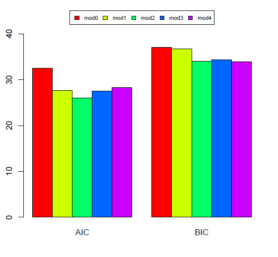
Model 2 is "the best", according to both AIC and BIC criteria. Mixed effects model comparison shows the general relevance of Vegetation and Sediment in determining the biodiversity variation. We now look again at the summary and verify if residuals of the chosen model are gaussian
> summary(mod2.delta)
Linear mixed-effects model fit by maximum likelihood Data: env
| AIC | BIC | logLik |
| 26.01904 | 33.9675 | -6.009521 |
Random effects: Formula: ~1 | sys
| (Intercept) | |
| StdDev: | 3.687605e-06 |
Formula: ~1 | lag %in% sys
| (Intercept) | Residual | |
| StdDev: | 8.330385e-07 | 0.3142222 |
Fixed effects: alpha.1 ~ Vegetation
| Value | Std.Error | DF | t-value | p-value | |
| (Intercept) | 1.4047387 | 0.1728598 | 11 | 8.126464 | 0.0000 |
| Vegetationmacroa | 0.7110108 | 0.2231610 | 11 | 3.186089 | 0.0087 |
| Vegetationnone | 0.4662216 | 0.2077516 | 11 | 2.244130 | 0.0464 |
| Vegetationsmacroph | -0.0252748 | 0.2444606 | 6 | -0.103390 | 0.9210 |
Correlation: |
|||||
| (Intr) | Vgttnm | Vgttnn | |||
| Vegetationmacroa | -0.775 | ||||
| Vegetationnone | -0.832 | 0.645 | |||
| Vegetationsmacroph | -0.707 | 0.548 | 0.588 |
Standardized Within-Group Residuals:
| Min | Q1 | Med | Q3 | Max |
| -2.7078336 | -0.3333537 | 0.1886809 | 0.5629413 | 1.9458803 |
Number of Observations: 23 Number of Groups:
| sys | lag | %in% | sys |
| 3 | 10 |
> qqnorm(residuals(mod2.delta))
> qqline(residuals(mod2.delta),col=2)
> shapiro.test(residuals(mod2.delta)) ### confirmed residuals are gaussian
Shapiro-Wilk normality test
data: residuals(mod2.delta)
W = 0.9383, p-value = 0.1651
To asses the random effects contribution to the alpha entropy measure, ob- serve the standard deviations given in the summary of the model
> ss=c(3.691927e-06,8.342304e-07)
> names(ss)=c("system","lagoon")
> barplot(ss,beside=T,col=c(5,3))
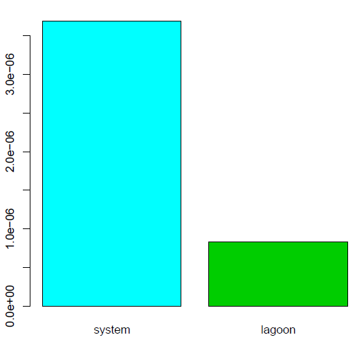
The graph above shows that the system level is the most relevant for these data. The use of mixed models facilitates the understanding of the spatial scale influence on biodiversity. Results emphasize that, in the Po river Delta, biodiversity conservation of lagoon ecosystems cannot be managed locally but, to be effective, requires a large scale process of governance.
Il delta del fiume Po: Modelli ad effetti misti (Mixed effects models)
Si è interessati alla determinazione quale scala spaziale (ecosistema, laguna o stazione di monitoraggio) sembra piú rilevante in termini di rappresentazione della variazione della biodiversitá. Gli effetti fissi sono dati dai fattori Vegetation (vegetazione) e Sediment (sedimento) che descrivono l'ambiente della stazione. Siccome sono variabili esplicative categoriche, la loro inclusione nella parte fissa del modello implica che verrá stimata un'intersezione fissa per ogni combinazione delle categorie, piú gli effetti casuali dei fattori System(sistema) e Lagoon (laguna). Per confronto, si considera un modello senza variabili esplicative, includendo solo una intersezione fissa e intersezioni casuali guidate dagli effetti annidati di System(sistema) e Lagoon (laguna). Effetti annidati sono rappresentati dalla sintassi effect1/effect2/effect3....
> require(nlme)
> alpha.1=delta.part$CommunityAlphaEntropies
> sys=env$System
> lag=env$Lagoon
> mod0.delta=lme(alpha.1~1,random=~1|sys/lag,data=env,method="ML")
> summary(mod0.delta)
Linear mixed-effects model fit by maximum likelihood
Data: env
| AIC | BIC | logLik |
| 32.47187 | 37.01384 | -12.23593 |
Random effects:
Formula: ~1 | sys
(Intercept)
StdDev: 7.931876e-06
Formula: ~1 | lag %in% sys
(Intercept) Residual
StdDev: 0.2696757 0.3427638
Fixed effects: alpha.1 ~ 1
| Value | Std.Error | DF | t-value | p-value | |
| (Intercept) | 1.723163 | 0.1172432 | 13 | 14.69735 | 0 |
Standardized Within-Group Residuals:
| Min | Q1 | Med | Q3 | Max |
| -1.7897264 | -0.4813381 | 0.1724562 | 0.5263777 | 1.3500645 |
Number of Observations: 23
Number of Groups:
| sys | lag | %in% | sys |
| 3 | 10 |
Si stima il modello includendo le due variabili esplicative: Vegetation e Sediment
> mod1.delta=lme(alpha.1~Vegetation+Sediment,random=~1|sys/lag,data=env,method="ML")
> summary(mod1.delta)
Linear mixed-effects model fit by maximum likelihood
Data: env
| AIC | BIC | logLik |
| 27.68141 | 36.76536 | -5.840703 |
Random effects: Formula: ~1 | sys
| (Intercept) | |
| StdDev: | 5.495947e-06 |
Formula: ~1 | lag %in% sys
| (Intercept) | Residual | |
| StdDev: | 1.127679e-06 | 0.3119242 |
Fixed effects: alpha.1 ~ Vegetation + Sediment
| Value | Std.Error | DF | t-value | p-value | |
| Intercept) | 1.4047387 | 0.1762978 | 11 | 7.967989 | 0.0000 |
| Vegetationmacroa | 0.7110108 | 0.2275994 | 11 | 3.123957 | 0.0097 |
| Vegetationnone | 0.4233437 | 0.2275994 | 11 | 1.860039 | 0.0898 |
| Vegetationsmacroph | -0.0252748 | 0.2493227 | 5 | -0.101374 | 0.9232 |
| Sedimentsand | 0.1286338 | 0.2493227 | 5 | 0.515933 | 0.6279 |
| Correlation: | |||||
| (Intr) | Vgttnm | Vgttnn | Vgttns | ||
| Vegetationmacroa | -0.775 | ||||
| Vegetationnone | -0.775 | 0.600 | |||
| Vegetationsmacroph | -0.707 | 0.548 | 0.548 | ||
| Sedimentsand | 0.000 | 0.000 | -0.365 | 0.000 |
Standardized Within-Group Residuals:
| Min | Q1 | Med | Q3 | Max |
| -2.5903194 | -0.5126984 | 0.1900709 | 0.6213941 | 1.9602155 |
Number of Observations: 23 Number of Groups:
| sys | lag | %in% | sys |
| 3 | 10 |
Si noti che solo alcune delle categorie di Vegetation e Sediment sono menzionati esplicitamente, si parla quindi di parametrizzazione corner-point, alcune categorie di riferimento sono associate all'intersezione generica e la differenze fra queste e le altre viene valutata. Successivamente nel riepilogo del modello mod1.delta si avrà un corner-point che è la combinazione delle categorie "emerged macrophytes" e "mud", mentre gli altri coefficienti misurano la differenza con il corner-point. Il livello "macroa" (presenza di macroalghe) differisce coerentemente dal corner-point, alcune differenze sono ache osservate per il livello "none", mentre la categoria del sedimento "sand" sembra non cambi significativamente rispetto al corner-point. Ora si provano modelli differenti
> mod2.delta=lme(alpha.1~Vegetation,random=~1|sys/lag,data=env,method="ML")
> summary(mod2.delta)
Linear mixed-effects model fit by maximum likelihood Data: env
| AIC | BIC | logLik |
| 26.01904 | 33.9675 | -6.009521 |
Random effects: Formula: ~1 | sys
| (Intercept) | |
| StdDev: | 3.687605e-06 |
Formula: ~1 | lag %in% sys
| (Intercept) | Residual | |
| StdDev: | 8.330385e-07 | 0.3142222 |
Fixed effects: alpha.1 ~ Vegetation
| Value | Std.Error | DF | t-value | p-value | |
| (Intercept) | 1.4047387 | 0.1728598 | 11 | 8.126464 | 0.0000 |
| Vegetationmacroa | 0.7110108 | 0.2231610 | 11 | 3.186089 | 0.0087 |
| Vegetationnone | 0.4662216 | 0.2077516 | 11 | 2.244130 | 0.0464 |
| Vegetationsmacroph | -0.0252748 | 0.2444606 | 6 | -0.103390 | 0.9210 |
| Correlation: | |||||
| (Intr) | Vgttnm | Vgttnn | |||
| Vegetationmacroa | -0.775 | ||||
| Vegetationnone | -0.832 | 0.645 | |||
| Vegetationsmacroph | -0.707 | 0.548 | 0.588 |
Standardized Within-Group Residuals:
| Min | Q1 | Med | Q3 | Max |
| -2.7078336 | -0.3333537 | 0.1886809 | 0.5629413 | 1.9458803 |
Number of Observations: 23
Number of Groups:
| sys | lag | %in% | sys |
| 3 | 10 |
Nel precedente riepilogo sembra che le differenzi piú forti in termini di effetti fissi si trovano fra le stazioni con macroalghe e quelle senza. Quindi si crea un fattore discriminante di presenza/assenza delle macroalghe e si include il fattore Sediment nel modello
> Macroa=ifelse(env$Vegetation=="macroa",1,0)
> Macroa=factor(Macroa)
> mod3.delta=lme(alpha.1~Macroa+Sediment,random=~1|sys/lag,data=env,method="ML")
> summary(mod3.delta)
Linear mixed-effects model fit by maximum likelihood Data: env
| AIC | BIC | logLik |
| 27.55772 | 34.37068 | -7.778858 |
Random effects: Formula: ~1 | sys
| (Intercept) | |
| StdDev: | 0.1882284 |
Formula: ~1 | lag %in% sys
| (Intercept) Residual | ||
| StdDev: | 9.551436e-06 | 0.3123423 |
Fixed effects: alpha.1 ~ Macroa + Sediment
| Value | Std.Error | DF | t-value | p-value | |
| (Intercept) | 1.5943983 | 0.1471106 | 12 | 10.838092 | 0.0000 |
| Macroa1 | 0.6161267 | 0.1777641 | 12 | 3.465978 | 0.0047 |
| Sedimentsand | 0.5193027 | 0.2310926 | 6 | 2.247162 | 0.0657 |
| Correlation: | |||||
| (Intr) | Macro1 | ||||
| Macroa1 | -0.304 | ||||
| Sedimentsand | -0.229 | 0.343 |
Standardized Within-Group Residuals:
| Min | Q1 | Med | Q3 | Max |
| -2.46104568 | -0.45583848 | -0.00266506 | 0.61053742 | 1.47064380 |
Number of Observations: 23
Number of Groups:
| sys | lag | %in% | sys |
| 3 | 10 |
Per aggiungere un altro termine di paragone, si stima il modello con solo il fattore Macroa come effetto fisso. Quindi si raccolgono i criteri AIC e BIC e si sceglierá il modello migliore in termini statistici.
> mod4.delta=lme(alpha.1~Macroa,random=~1|sys/lag,data=env,method="ML")
> comp=data.frame(AIC=c(
+ AIC(mod0.delta),
+ AIC(mod1.delta),
+ AIC(mod2.delta),
+ AIC(mod3.delta),
+ AIC(mod4.delta)
+ ), BIC=c(
+ BIC(mod0.delta),
+ BIC(mod1.delta),
+ BIC(mod2.delta),
+ BIC(mod3.delta),
+ BIC(mod4.delta)
+ ))
> row.names(comp)=c("mod0","mod1","mod2","mod3","mod4")
> barplot(as.matrix(comp),beside=T,col=rainbow(5),legend=T,
+ args.legend=list(horiz=T,x="top",cex=0.7),ylim=c(0,45))
Il modello 2 é il "migliore", secondo i criteri AIC e BIC. Il confronto di modelli ad effetti misti mostra la rilevanza generale della vegetazione (Vegetation) e del sedimento (Sediment) nella determinazione della biodiversitá. Si dia uno sguardo al riepilogo e si verifichi se i residui del modello scelto seguono una distribuzione gaussiana.
> summary(mod2.delta)
Linear mixed-effects model fit by maximum likelihood Data: env
| AIC | BIC | logLik |
| 26.01904 | 33.9675 | -6.009521 |
Random effects: Formula: ~1 | sys
| (Intercept) | |
| StdDev: | 3.687605e-06 |
Formula: ~1 | lag %in% sys
| (Intercept) | Residual | |
| StdDev: | 8.330385e-07 | 0.3142222 |
Fixed effects: alpha.1 ~ Vegetation
| Value | Std.Error | DF | t-value | p-value | |
| (Intercept) | 1.4047387 | 0.1728598 | 11 | 8.126464 | 0.0000 |
| Vegetationmacroa | 0.7110108 | 0.2231610 | 11 | 3.186089 | 0.0087 |
| Vegetationnone | 0.4662216 | 0.2077516 | 11 | 2.244130 | 0.0464 |
| Vegetationsmacroph | -0.0252748 | 0.2444606 | 6 | -0.103390 | 0.9210 |
Correlation: |
|||||
| (Intr) | Vgttnm | Vgttnn | |||
| Vegetationmacroa | -0.775 | ||||
| Vegetationnone | -0.832 | 0.645 | |||
| Vegetationsmacroph | -0.707 | 0.548 | 0.588 |
Standardized Within-Group Residuals:
| Min | Q1 | Med | Q3 | Max |
| -2.7078336 | -0.3333537 | 0.1886809 | 0.5629413 | 1.9458803 |
Number of Observations: 23 Number of Groups:
| sys | lag | %in% | sys |
| 3 | 10 |
> qqnorm(residuals(mod2.delta))
> qqline(residuals(mod2.delta),col=2)
> shapiro.test(residuals(mod2.delta)) ### confirmed residuals are gaussian
Shapiro-Wilk normality test
data: residuals(mod2.delta)
W = 0.9383, p-value = 0.1651
Per valutare il contributo degli effetti casuali alla misura dell'entropia alfa, é necessario osservare le deviazioni standard indicate nel riepilogo del modello
> ss=c(3.691927e-06,8.342304e-07)
> names(ss)=c("system","lagoon")
> barplot(ss,beside=T,col=c(5,3))
Il grafico mostra che il livello "sistema" è il piú importante per questi dati. L'uso dei modelli misti facilita la comprensione dell'influenza spaziale sulla biodiversitá. I risultati moeetono alla luce che, per quanto riguarda il delta del fiume Po, la conservazione dell'ecosistema lagunare non puó essere gestito localmente ma, per essere efficae, richiede una gestione sistematica su larga scala.