Introduction to R - Introduzione a R
| Site: | LifeWatch ERIC Training Platform |
| Course: | Introduction to partitioning and mixed models for biodiversity analysis in R |
| Book: | Introduction to R - Introduzione a R |
| Printed by: | Guest user |
| Date: | Tuesday, 15 September 2026, 2:26 PM |
Description
Introduction to R - Introduzione a R
Table of contents
- 1. What is R?Cos'è R?
- 2. R Installation Installazione di R
- 3. The first session with RLa prima sessione con R
- 4. Getting HelpOttenere aiuto
- 5. Close and save our work in the working directoryChiusura e salvataggio nella cartella di lavoro
- 6. Packages: how to load and install themPacchetti: come caricarli ed installarli
- 7. R objectsGli oggetti di R
- 8. Read data from a text fileLeggere dati da un file di testo
- 9. Some simple graphicsAlcuni grafici semplici
- 10. Final TipsSuggerimenti finali
What is R?
R is an integrated suite of software facilities for data manipulation, calculation and graphical display. It is an open source software developed by the statistical community world wide. The latter ensures high scientic quality of implemented tools and a constant peer-review of R proposed procedures. With R we can perform effective data handling and store data, we can use graphical facilities for data analysis and display either directly at the computer or on hardcopy. We can develop our own procedures using a well-established and effective programming language. R has some peculiarities, it does not have a standard graphical interface, it works using command lines. There exist several graphical interfaces, most are specific for an operating system. If one should be recommended we'd chose Rstudio that is available for all OS. In what follows we'll illustrate R usage without graphical interface using scripts and the R console. There is an important difference in philosophy between R and the other main statistical systems. In R a statistical analysis is normally done as a series of steps with intermediate results stored in objects. Whereas SAS and SPSS provide output files with several details as results of a data analysis, R provides minimal output and stores the results in a fit object for subsequent calls by functions such as summary.
R is organized with several modules, in the installation binaries one gets the base set of packages, it contains a large variety of statistical and graphical tools that allow the elaboration of most basic data analysis. It is possible for example to fit a linear models, generalized linear models (GLM) and log linear models, perform a simple principal component analysis or an ANOVA. Then hundreds of packages implementing graphical or modeling tools are available. If for example it is of interest to estimate a Generalized Additive Model (GAM) it is necessary to load the mgcv or the gam package. Once the R is installed locally it is possible to download and install packages
Cos'é R?
R é una suite integrata di risorse software per la manipolazione dei dati, calcolo e visualizzazione grafica. É un software open source sviluppato dalla community di statistica in tutto il mondo. Il chè assicura un'alta qualitá scientifica degli strumenti implementati e una constante revisione delle procedure proposte per R. Con R é possibile eseguire manipolazione dati e immagazzinamento degli stessi, si possono utilizzare risorse grafiche per le analisi dei dati e visualizzarli direttamente sul computer o su supporto cartaceo. É possibile sviluppare le prorprie procedure utilizzando un linguaggio consolidato ed efficiente. R presenta alcune peculiaritá, non ha una interfaccia grafica, si utilizza da riga di comando. Vi sono diverse interfaccie grafiche, la maggior parte sono specifiche per il singolo sistema operativo. Se si deve suggerire un'interfaccia grafica, la scelta cade sicuramente su RStudio, che é disponibile per tutti i sistemi operativi. in questo corso si illustrerá l'uso di R senza interfaccia grafica, utilizzando scripts la console di R. Vi é una importante differenza nella filosofia tra R e i maggiori sistemi statistici. In R un'analisi statistica é normalmente eseguita come una serie di passi (step) dove i risultati intermedi sono immagazzinati in oggetti. Mentre SAS e SPSS forniscono un file in output dettagliato come risultato di un'analisi di dati, R fornisce output minimi e immagazzina i risultati in un adeguato oggetto disponibile per essere richiamato da altre funzioni come summary.
R é composto da diversi moduli, nei file di installazione é presente un set di base di pacchetti (packages), che contiene una grande varietá di strumenti statistici e grafici che permettono l'elaborazione della maggior parte di analisi di base. É possibile, per esempio, calcolare modelli lineari, modelli lineari generalizzati (GLM) e monitorare modelli lineari, eseguire una semplice analisi di componenti principali o un analisi di varianza (ANOVA). Sono disponibili centinaia di ulteriori pacchetti per l'implementazioni grafiche e strumenti per la modellazione. Se, per esempio, si vuole stimare un modello additivo generalizzato (Generalized Additive Model - GAM) é necessario il pacchetto mgcv oppure il pacchetto gam. Un volta installato R localmente é possibile scaricare e installare i pacchetti necessari.
R Installation
R can be installed on any OS (Windows, Linux, MAC OS) The binaries for installation can be downloaded from http://www.r-project.org/
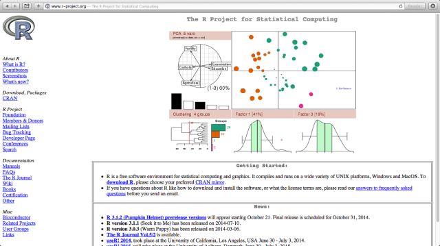
Figure 1: R web site
To install R first one goes on the left menu on the R-project web page and clicks on CRAN, there it is possible to select a mirror server (it is best to select the closest to ones current location). From the selected mirror it is possible to download all the required binaries and installation documentation. For frequently asked question the following link is useful: http://cran.mirror.garr.it/mirrors/CRAN/faqs.html
Assuming the installation of R is terminated we move to the first R session.
In our first session we are going to use features available from the base module
We'll learn:
-
- how to start and end a session,
- how to read data from a text file (or a csv)
- how to compute basic descriptive statistics
- how to handle plots
Then let's start
Installazione di R
R puó essere installato in ogni sistema operativo (Windows, Linux, MAC OS). I file di installazione possono essere scaricati da http://www.r-project.org/
Figura 1: Sito del progetto R
Per installare R, selezionare CRAN dal menu del sito di R-project, successivamente é necessario selezionare un server dal quale scaricare i file di installazione (si suggerisce di selezionare uno vicino alla propria posizione). Dal server selezionato é e possibile scaricare anche la documentazione per l'installazione. Per le domande frequenti (FAQ) si utilizza il seguente link: http://cran.mirror.garr.it/mirrors/CRAN/faqs.html
Una volta terminata l'installazione di R, si partirá con la prima sessione di R.
Nella prima sessione si utilizzeranno le risorse disponibili nel modulo base
Nello specifico, si apprenderá:
- come iniziare e terminare una sessione,
- come leggere dati da un file di testo (o un file csv),
- come effettuare statistiche descrittive di base
- come gestire i grafici
Si proceda!
The first session with R
Now double click on the R icon and follow the tutorial by typing commands as shown below, on the R console.
We can start using R as a calculator
> 2+2
[1] 4
The standard assignment operator in R is > − or =. You can use both symbols indiscriminately.
R works using objects and it is case sensitive, then an object named a and an object named A, are two different things. If we type the name of an object that has not already been created we get an error message telling us that the object does not exist in the current work space.
> a=2+2
> a
[1] 4
> b=2*a
In R most of the work is going to be organized as follows:
- Open the R console.
- Read data into the work space.
- Start elaborations and as the work proceeds, save effective commands into a script.
- Save data and elaboration together with the script file in a working directory.
The script file is a simple text file that will contain all the commands necessary to perform the desired task on the data. It can be opened into the R work session using the R internal editor. From the editor it is possible to directly select and execute command lines. In the windows installation this is obtain using ctrl+r and in the MacOs using cmd+enter. It is useful to write comments in the script file so to keep track of the analysis and to ease the file readability. To write comments in the command script we use the symbol # , any word written after # will not be executed.
La prima sessione con R
Per lanciare R fare doppio click sull'icona di R, si segua il tutorial digitando i comandi che seguono nella console di R.
Uso di R come calcolatrice
> 2+2
[1] 4
L'operatore di assegnazione in R é > − or =. Si possono usare indistintamente entrambi.
R usa gli oggetti ed distingue le maiuscole dalle minuscole (case-sensitive), quindi un oggetto chiamato a e un oggetto chiamato A, sono due oggetti differenti. Se si digita il nome di un oggetto che non é stato ancora creato si otterá un errore che indica che l'oggetto richiesto non esiste nello spazio di lavoro corrente.
> a=2+2
> a
[1] 4
> b=2*a
La maggior parte del lavoro in R sará organizzato nel seguente modo:
- Si apre la console di R.
- Si importano i dati nello spazio di lavoro.
- Si effettuano le elaborazioni e man mano che il lavoro procede, si salvano i comandi efficaci un file di script.
- Infine si salvano i dati e le elaborazioni insieme in un file di script in una directory di lavoro.
Il file di script é un semplice file di testo contenete tutti i comandi necessari per eseguire una determinata elaborazione sui dati. Puó essere modificato dalla sessione di lavoro di R con l'editor interno di R. Dall'editoe é possibile selezionare direttamente ed eseguire righe di comando. Nell'installazione di Windows si usa ctrl+r e in quella di MacOs si usa cmd+enter. É utile aggiungere dei commenti nello script in modo da tenere traccia dell'analisi e per facilitare la leggibilitá del file. Per inserire dei commenti nello script dei comandi si usa il simbolo #, qualunque parola scritta dopo # non sará eseguita.
Getting Help
Several resources are available to help you learn more about R. These include several facilities WITHIN R itself and, of course, on the Web. The help() allows to find information of a given function for example mean by typing
> help(mean)
or
> ?mean
For special characters and some reserved words one has to use quote For example, if you have problems with < operator type
> help("<")
For example, if the problem is with the reserved word if (basic control-flow constructs see later), type
> ?"if"
The example() function will isolate the examples in the help page for the given function.
> example(mean)
mean> x <- c(0:10, 50)
mean> xm <- mean(x)
mean> c(xm, mean(x, trim = 0.10))
[1] 8.75 5.50
> example("if")
if> for(i in 1:5) print(1:i)
[1] 1
[1] 1 2
[1] 1 2 3
[1] 1 2 3 4
[1] 1 2 3 4 5
if> for(n in c(2,5,10,20,50)) {
if+ x <- stats::rnorm
if+ cat(n, ": ", sum(x^2), "\n", sep = "")
if+ }
2: 0.2666525
5: 3.512141
10: 8.711755
20: 12.94274
50: 52.22404
if> f <- factor(sample(letters[1:5], 10, replace = TRUE))
if> for(i in unique(f)) print(i)
[1] "e"
[1] "b"
[1] "a"
[1] "c"
[1] "d"
The help.search() function finds information when the help() and example() functions fail or one doesn't know what exactly what to look for. It is a Google- style search through R documentation. For instance, say you need a function to draw three-dimensional plots. Type help.search('3d plots') R finds the packages that could contain functions for drawing 3d plots ... however it takes just forever to find them locally! Use the web instead.
R is organized in packages or library as illustrated in more details in section 2.3. To learn about entire packages it is enough to type help(package=PACKAGE's NAME). For example, for the package "graphics"
> help(package=graphics)
while to get the list of all commands and datasets in a package just type library(help=name of the package)
> library(help=graphics)
Notice that all the commands introduced in this text are available as session script and there more examples of help search are reported.
Ottenere aiuto
Diverse risorse sono disponibili per conoscere meglio l'ambiente di R. Queste comprendono risorse INCLUSE in R e, ovviamente, sul Web. La funzione help() consente di reperire informazioni su un'altra funzione, come ad esempio la funzione mean(media).
> help(mean)
oppure
> ?mean
Per quanto riguarda caratteri speciali o parole riservate é necessario usare le virgolette ("). Per esempio se si vuole aiuto per l'operatore < si digita
> help("<")
Per esempio, se si ha un problema con la parola riservata if (controllo di flusso base), digitare
> ?"if"
La funzione example() estrae gli esempi dalla pagina di help per una data funzione:
> example(mean)
mean> x <- c(0:10, 50)
mean> xm <- mean(x)
mean> c(xm, mean(x, trim = 0.10))
[1] 8.75 5.50
> example("if")
if> for(i in 1:5) print(1:i)
[1] 1
[1] 1 2
[1] 1 2 3
[1] 1 2 3 4
[1] 1 2 3 4 5
if> for(n in c(2,5,10,20,50)) {
if+ x <- stats::rnorm
if+ cat(n, ": ", sum(x^2), "\n", sep = "")
if+ }
2: 0.2666525
5: 3.512141
10: 8.711755
20: 12.94274
50: 52.22404
if> f <- factor(sample(letters[1:5], 10, replace = TRUE))
if> for(i in unique(f)) print(i)
[1] "e"
[1] "b"
[1] "a"
[1] "c"
[1] "d"
La funzione help.search() trova informazioni quando le funzioni help() e example() non riescono a reperire informazioni adeguate o si ha la necessitá di fare una ricerca piú libere. Si tratta di una ricerca, stile Google, effettuata in tutta la documentazion di R. Ad esempio, si ha bisogno di una funzione che disegna grafici (plot) 3D. Si digita help.search('3d plots') e R trova tutti i pacchetti che consento il disegno di grafici 3D ... comunque, alcune volte la ricerca in locale é molto lunga! Usare per le ricerche il web.
R é organizzato in pacchetti o librerie, come si vedrá in dettaglio nella sezione successiva. Per conoscere tutto di un pachetto é sufficiente digitare help(package=NOME PACCHETTO). Per esempio, per il pacchetto "grphics"
> help(package=graphics)
mentre per avere un elenco di tutti i comandi e i dataset presenti in un pacchetto é sufficiente digitare library(help=NOME PACCHETTO)
> library(help=graphics)
Si tenga presente che tutti i comandi usati in questa sezione sono disponibili come script di sessione, dove sono presenti ulteriori esempi sulle ricreche di help.
Close and save our work in the working directory
First of all verify which is the working directory. The getwd() function let one knows where the sessions currently located on the hard disk
> getwd()
[1] "/Dropbox/tutorial partitioning/IntroduzioneR"
to change working directory one can use the R console or the menu, using the R console requires to know the system path to the working directory, notice that R uses the Linux convention to describe patterns, it uses / instead of \ to separate directories in the path. The function setwd() allows to set the working directory using the syntax setwd(``tutorial/IntroductionToR')'. Once the working directory has been set, it is possible to save the objects created in the current work space. To see which objects are in the work space use the command ls()
> ls()
[1] "a" "b" "f" "i" "n" "x" "xm"
To save all objects use the save.image function, the syntax is save.image("filename.RData"), the .RData extension is mandatory and identifies the R data format. By double clicking on .RData files R opens and sets as working directory the one containing the data file. Then it is very convenient to establish one working directory for each project and keep in it data, scripts and related outputs.
Chiusura e salvataggio nella cartella di lavoro
Inanzitutto si verifica la cartella di lavoro corrente. La funzione getwd() restituisce l'ubicazione della cartella di lavoro corrente
> getwd()
[1] "/Dropbox/tutorial partitioning/IntroduzioneR"
per cambiare la cartella di lavoro si puó utilizzare la console di R o il menu, se si utilizza la console di R é necessario conoscere il percorso di sistema alla cartella di lavoro, si tenga presente che R utilizza la convenzione di Linux per la descrizione dei percorsi, ossia utilizza "/" invece di "\" per separare le cartelle nel percorso. la funzione setwd() consente di impostare la cartella di lavoro con la sintassi setwd("tutorial/IntroductionToR"). Una volta impostata la cartella di lavoro, é possibile salvare gli oggetti creati nello spazio di lavoro corrente. Per vedere quali oggetti sono presenti nello spazio di lavoro si usa il comando ls()
> ls()
[1] "a" "b" "f" "i" "n" "x" "xm"
Per salvare tutti gli oggetti utilizzare la funzione save.image(), la sintassi é save.image("NOMEFILE.RData"), l'estensione .RData é obbligatoria ed identifica il formato dati di R. Facendo doppio click su un file .RData, R apre ed imposta la cartella di lavoro quella in cui é contenuto il file. É molto utile utilizzare una cartella di lavoro per ogni progetto e che contenga dati, script e relativi output.
Packages: how to load and install them
In order to install and make use of packages you first have to find them. Luckily, most (but not all) R packages are organized and available from CRAN-the Comprehensive R Archive Network. Just click on the Packages link to see the full list of contributed packages. Packages are listed alphabetically with a short description. Unfortunately, there is no rating system but you can get a quick sense of quality by clicking on a package link and looking at the "Published" date and especially any "Reverse dependencies" listed at the the bottom of a package. Reading the documentation and looking at the number of releases in the "Old sources" is also very helpful. CRAN also maintains a set of Task Views that identify all the packages associated with a particular task. The maintainers of these views do a generally excellent job of staying on top of their area of interest and giving a detailed summary of which packages do what. The basics of package installation are given in chapter 6 of R Installation and Administration. From the command line the fuction install.packages allows packages installation, the syntax is install.packages(package name, dependencies=TRUE). The option dependencies tells the installation routine to install the package and any other package to which this one is connected. An easier alternative is to use the package manager available from the R console menu, in the MAC OS installation remember to check the dependencies option in the installation menu. The function installed.packages() allows to verify which packages are installed on the computer. To make a package available during the current session it is necessary to recall it and this can be done using the Console menu or the function library(package name). For example typing
> library(entropart)
it makes the package entropart available during the session. Our suggestion is to install using the menu (remember the dependencies) and to recall packages using library
Pacchetti: come caricarli ed installarli
Per poter installare ed usare i pacchetti é necessario trovarli. Fortunatamente, la maggior parte (ma non tutti) i pacchetti di R sono elencati e disponibile su CRAN (Comprehensive R Archive Network). L'elenco completo é disponibile con un semplce click su "Packages". I pacchetti sono elencati con una breve descrizione. Sfortunatamente, non é presente un sistema di valutazione (rating), ma ci si puó fare un'idea della qualitá del pacchetto cliccando su di esso e osservando la data di pubblicazione ("Published") e, in particolare, le dipendenze da altri pacchetti ("Reverse dependencies") evidenziati alla fine della descrizione del pacchetto. Anche leggere la documentazione e verificando il numero di release alla voce "Old sources" é molto utile. CRAN detiene un elenco di "Task Views" che identificano tutti pacchetti associati ad una particolare attivitá (task). I manutentori di queste "Views" generalmente fanno un lavoro eccellente nell'aggiornamento della propria area d'interesse e fornendo un riepilogo dettagliato su quali pacchetti fanno cosa. Le istruzioni base sull'installazione di pacchetti sono descritte nel capitolo 6 del manuale di Installazione e amministrazione di R ("R Installation and Administration"). L'installazione dei pacchetti viene eseguita tramite la funzione install.packages(), la sintassi é install.packages(nome pacchetto,dependencies=TRUE). Il parametro dependencies indica alla routine di installare il pacchetto e ogni altro pacchetto a cui é legato. Un'alternativa piú semplice é qualla di utilizzare il gestore di pacchetti ("package manager") disponibile dal menu della console di R, nell'installazione su MAC OS é necessario "spuntare" l'opzione delle dipendenze nel menu d'installazione. La funzione installed.packages() permette di verificare quali pacchetti sono installati sul computer. Per rendere un pacchetto disponibile nella sessione di lavoro corrente é necessario richiamarlo ed é possibile farlo tramite il menu di console o tramite la funzione library(nome pacchetto). Per esempio
> library(entropart)
rende il pacchetto entropart disponibile per la sessione.
Si suggerisce di installare i pacchetti tramite menu (si ricordino le dipendenze) e di richiamrli utilizzando library().
R objects
R objects types are called modes. In the next paragraphs we will see different R modes. The simplest R objects and their modes are:
- MODE: NUMERIC (numeric [integer, real] or complex)
> a=10
> b=15.53
> d=3.51+1.2i
check the mode of the objects by typing
> mode(a)
[1] "numeric"
> mode(b)
[1] "numeric"
> mode(d)
[1] "complex"
- MODE: CHARACTERS
> e="Hallo"
> f="World"
> mode(e)
[1] "character"
- MODE: LOGICAL
> g=TRUE
> h=FALSE
> i=F
> l=T
> mode(g)
[1] "logical"
- VECTORS: Vectors are created using the concatenating function c. For example a vector of numbers
> v1=c(5,2,3,1,9)
> v1
[1] 5 2 3 1 9
> mode(v1)
[1] "numeric"
A vector of characters
> v2=c("a","b","c")
> v2
[1] "a" "b" "c"
> mode(v2)
[1] "character"
A vector of "objects"
> v3=c(a,b,d)
> v4=c(g,h,i,l)
> mode(v4)
[1] "logical"
and an empty vector
> v5=c()
Individual elements of a vector are accessed via [position of the element]. For example to select the second element of v1, type
> v1[2] [1] 2
Subsetting is a very important operation on vectors. For example to select a subset of consecutive elements of the vector type [position of the first element:position of the last element]. For example, if you want to select from the second to the fourth element of v1
> v1[2:4]
[1] 2 3 1
> v1
[1] 5 2 3 1 9
To select elements in non consecutive positions type their positions in the vector using the c() function. For example, to select elements of position 3,2,5 of v1
> v1[c(3,2,5)]
[1] 3 2 9
to know how many elements are in a vector type
> length(v1) [1] 5
Simple operations on vector can be carried on such as:
> sum(v1)
[1] 20
> mean(v1)
[1] 4
> prod(v1)
[1] 270
> cumsum(v1)
[1] 5 7 10 11 20
> v1-2
[1] 3 0 1 -1 7
> v1/2
[1] 2.5 1.0 1.5 0.5 4.5
When applying an operation to two vectors that requires them to be of the same length, R automatically recycles, or repeats, the shorter one, until it is long enough to match the longer one
> c(2,4,1)+c(5,1,2,0,0,4)
[1] 7 5 3 2 4 5
that is equal to
> c(2,4,1,2,4,1)+c(5,1,2,0,0,4)
[1] 7 5 3 2 4 5
> v1*c(5,2)
[1] 25 4 15 2 45
equivalent to
> v1*c(5,2,5,2,5)
[1] 25 4 15 2 45
Vectors contain objects of the same mode. If one concatenates elements of different modes, for example numeric and character the result is
> new.1=c(v1,v2)
> mode(new.1)
[1] "character"
> new.2=c(v1,v2,v3,g,h,v4)
> new.2
| [1] | "5" | "2" | "3" | "1" | "9" | "a" | "b" | "c" |
| [9] | "10+0i" | "15.53+0i" | "3.51+1.2i" | "TRUE" | "FALSE" | "TRUE" | "FALSE" | "FALSE" |
| [17] | "TRUE" |
> mode(new.2)
[1] "character"
It is always possible to change the mode of a vector
> as.character(v1)
[1] "5" "2" "3" "1" "9"
> as.character(v3)
[1] "10+0i" "15.53+0i" "3.51+1.2i"
> as.character(v4)
[1] "TRUE" "FALSE" "FALSE" "TRUE"
> as.numeric(v4)
[1] 1 0 0 1
> as.numeric(v2)
[1] NA NA NA
- MODE: LIST One simple solution to put elements of different modes and lengths together without changing their modes or reciclying elements is the list. A list is a container for items of different data types. For example:
> list.1=list(c("Hallo","Friends","Hallo"),c(30,50,0.5,0.1),c(TRUE,TRUE,FALSE))
> list.1
[[1]]
[1] "Hallo" "Friends" "Hallo"
[[2]]
[1] 30.0 50.0 0.5 0.1
[[3]]
[1] TRUE TRUE FALSE
> mode(list.1) [1] "list"
To access list elements we have two solutions.
Solution 1: if the elements of the list do not have a name as in list.1, just type the position using [[]]
> list.1[[1]]
[1] "Hallo" "Friends" "Hallo"
> list.1[[1]][1]
[1] "Hallo"
> list.1[[1]][2]
[1] "Friends"
> list.1[[1]][c(1,3)]
[1] "Hallo" "Hallo"
> list.1[[2]]
[1] 30.0 50.0 0.5 0.1
> list.1[[2]][4]
[1] 0.1
> list.1[[2]][1:3]
[1] 30.0 50.0 0.5
> list.1[[2]][c(1,4)]
[1] 30.0 0.1
Solution 2: if the elements of the list have a name, you can directly access them using $
> list.2=list(welcome=c("Hallo","Friends","Hallo"),
+ mynumbers=c(30,50,0.5,0.1),
+ myidea=c(TRUE,TRUE,FALSE))
> list.2
$welcome
[1] "Hallo" "Friends" "Hallo"
$mynumbers
[1] 30.0 50.0 0.5 0.1
$myidea
[1] TRUE TRUE FALSE
> list.2[[1]]
[1] "Hallo" "Friends" "Hallo"
> # is equivalent to
> list.2$welcome
[1] "Hallo" "Friends" "Hallo"
> list.2[[1]][c(1,3)]
[1] "Hallo" "Hallo"
> list.2$welcome[c(1,3)]
[1] "Hallo" "Hallo"
Gli oggetti di R
I tipi di oggetto di R sono chiamati "modi". Nei seguentei paragrafi si vedranno diversi "modi" in R. Gli oggetti piú semplici ed i loro modi in R sono:
- MODO: NUMERICO (numeric [integer, real] or complex)
> a=10
> b=15.53
> d=3.51+1.2i
si verifica il modo di un oggetto digitando mode
> mode(a)
[1] "numeric"
> mode(b)
[1] "numeric"
> mode(d)
[1] "complex"
- MODO: CARATTERI
> e="Hallo"
> f="World"
> mode(e)
[1] "character"
- MODO: LOGICO
> g=TRUE
> h=FALSE
> i=F
> l=T
> mode(g)
[1] "logical"
- VETTORI: I vettori sono creati utilizzando la funzione di concatenazione c(). Per esempio un vettore di numeri
> v1=c(5,2,3,1,9)
> v1
[1] 5 2 3 1 9
> mode(v1)
[1] "numeric"
Un vettore di caratteri
> v2=c("a","b","c")
> v2
[1] "a" "b" "c"
> mode(v2)
[1] "character"
Un vettore di "oggetti"
> v3=c(a,b,d)
> v4=c(g,h,i,l)
> mode(v4)
[1] "logical"
e un vettore vuoto
> v5=c()
I singoli elementi di un vettore vengono richiamati utilizzando [position of the element]. Per selezionare il secondo elemento del vettore v1, si digita
> v1[2] [1] 2
Una operazione importante sui vettori é l'estrazione di sottoinsiemi. Per esempio per selezionare un sottoinsieme di elementi consecutivi di un vettore si utilizza [posizione del primo elemento:posizione dell'ultimo elemento]. Per esempio, se si vuole selezionare dal secondo al quarto elemento del vettore v1
> v1[2:4]
[1] 2 3 1
> v1
[1] 5 2 3 1 9
Per selezionare elementi in posizioni non consecutive é sufficiente digitare la loro posizione nel vettore utilizzare la funzione c(). Per esempio, per selezionare gli elementi nelle posizioni 3,2,5 di v1
> v1[c(3,2,5)]
[1] 3 2 9
per conoscere il numero di elementi in un vettore digitare
> length(v1) [1] 5
Si possono eseguire operazioni semplici sui vettori, come:
> sum(v1)
[1] 20
> mean(v1)
[1] 4
> prod(v1)
[1] 270
> cumsum(v1)
[1] 5 7 10 11 20
> v1-2
[1] 3 0 1 -1 7
> v1/2
[1] 2.5 1.0 1.5 0.5 4.5
Se si effettuano operazioni fra due vettori é necessario che siano della stessa grandezza. R automaticamente ripete il vettore piú piccolo fino a quando non ha la stessa lunghezza dell'altro
> c(2,4,1)+c(5,1,2,0,0,4)
[1] 7 5 3 2 4 5
che é uguale a
> c(2,4,1,2,4,1)+c(5,1,2,0,0,4)
[1] 7 5 3 2 4 5
> v1*c(5,2)
[1] 25 4 15 2 45
é equivalente a
> v1*c(5,2,5,2,5)
[1] 25 4 15 2 45
Vettori contengono oggetti dello stesso modo (tipo). Se si concatenano elemnti di modi diversi, come ad esempio numerico e carattere il risultato sará
> new.1=c(v1,v2)
> mode(new.1)
[1] "character"
> new.2=c(v1,v2,v3,g,h,v4)
> new.2
| [1] | "5" | "2" | "3" | "1" | "9" | "a" | "b" | "c" |
| [9] | "10+0i" | "15.53+0i" | "3.51+1.2i" | "TRUE" | "FALSE" | "TRUE" | "FALSE" | "FALSE" |
| [17] | "TRUE" |
> mode(new.2)
[1] "character"
É sempre possibile cambiare il modo di un vettore
> as.character(v1)
[1] "5" "2" "3" "1" "9"
> as.character(v3)
[1] "10+0i" "15.53+0i" "3.51+1.2i"
> as.character(v4)
[1] "TRUE" "FALSE" "FALSE" "TRUE"
> as.numeric(v4)
[1] 1 0 0 1
> as.numeric(v2)
[1] NA NA NA
- MODO: LISTA Una soluzione semplice per unire elementi di modi e di lunghezze diverse senza cambiare il loro modo o ripetendo gli elementi é la lista (list). Una lista é un contenitore di elementi di tipi di dati differenti. Per esempio:
> list.1=list(c("Hallo","Friends","Hallo"),c(30,50,0.5,0.1),c(TRUE,TRUE,FALSE))
> list.1
[[1]]
[1] "Hallo" "Friends" "Hallo"
[[2]]
[1] 30.0 50.0 0.5 0.1
[[3]]
[1] TRUE TRUE FALSE
> mode(list.1) [1] "list"
Per accedere agli elemnti di una lista ci sono due modalitá.
Modalitá 1: se gli elementi della lista non hanno nome, come nella lista list.1, é sufficiente indicare la posizione utilizzando [[]]
> list.1[[1]]
[1] "Hallo" "Friends" "Hallo"
> list.1[[1]][1]
[1] "Hallo"
> list.1[[1]][2]
[1] "Friends"
> list.1[[1]][c(1,3)]
[1] "Hallo" "Hallo"
> list.1[[2]]
[1] 30.0 50.0 0.5 0.1
> list.1[[2]][4]
[1] 0.1
> list.1[[2]][1:3]
[1] 30.0 50.0 0.5
> list.1[[2]][c(1,4)]
[1] 30.0 0.1
Modalitá 2: se gli elementi hanno un nome, si puó accedere agli elementi direttamente dal nome utilizzando $
> list.2=list(welcome=c("Hallo","Friends","Hallo"),
+ mynumbers=c(30,50,0.5,0.1),
+ myidea=c(TRUE,TRUE,FALSE))
> list.2
$welcome
[1] "Hallo" "Friends" "Hallo"
$mynumbers
[1] 30.0 50.0 0.5 0.1
$myidea
[1] TRUE TRUE FALSE
> list.2[[1]]
[1] "Hallo" "Friends" "Hallo"
> # is equivalent to
> list.2$welcome
[1] "Hallo" "Friends" "Hallo"
> list.2[[1]][c(1,3)]
[1] "Hallo" "Hallo"
> list.2$welcome[c(1,3)]
[1] "Hallo" "Hallo"
Read data from a text file
First of all verify how data are organized in the text file: is there a column header? which is the field separator (space, ",", ";")? which is the decimal delimiter (".", ",")? once these questions are answered we are ready to load data from a file present in the working directory
> dat=read.table("iris.txt",header=T,dec=".")
This data le contains the famous (Fisher's or Anderson's) iris data set, with the measurements in centimeters of the variables sepal length and width and petal length and width, respectively, for 50 flowers from each of 3 species of iris. The species are Iris setosa, versicolor, and virginica.
> dat1=read.table("iris.csv",header=T,sep=";")
using
> ?read.table
we can see all the options available to read text formatted data. to import data from databases (access, mysql etc.) there exist several packages such as RODBC (it connects to most existing databases including excel), foreign (to read .dbf, SAS, SPSS, Matlab and more).
> str(dat)
'data.frame': 150 obs. of 5 variables:
$ Sepal.Length: num 5.1 4.9 4.7 4.6 5 5.4 4.6 5 4.4 4.9 ...
$ Sepal.Width : num 3.5 3 3.2 3.1 3.6 3.9 3.4 3.4 2.9 3.1 ...
$ Petal.Length: num 1.4 1.4 1.3 1.5 1.4 1.7 1.4 1.5 1.4 1.5 ...
$ Petal.Width : num 0.2 0.2 0.2 0.2 0.2 0.4 0.3 0.2 0.2 0.1 ...
$ Species : Factor w/ 3 levels "setosa","versicolor",..: 1 1 1 1 1 1 1 1 1 1 ...
this function compactly displays the internal structure of an R object while
> summary(dat)
| Sepal.Length | Sepal.Width | Petal.Length | Petal.Width | Species | ||||||||||
| Min. : | 4.300 | Min. : | 2.000 | Min. : | 1.000 | Min. : | 0.100 | setosa : | 50 | |||||
| 1st Qu.: | 5.100 | 1st Qu.: | 2.800 | 1st Qu.: | 1.600 | 1st Qu.: | 0.300 | versicolor: | 50 | |||||
| Median : | 5.800 | Median : | 3.000 | Median : | 4.350 | Median : | 1.300 | virginica : | 50 | |||||
| Mean : | 5.843 | Mean : | 3.057 | Mean : | 3.758 | Mean : | 1.199 | |||||||
| 3rd Qu.: | 6.400 | 3rd Qu.: | 3.300 | 3rd Qu.: | 5.100 | 3rd Qu.: | 1.800 | |||||||
| Max. : | 7.900 | Max. : | 4.400 | Max. : | 6.900 | Max. : | 2.500 |
it returns basic statistics from the columns of the object dat. summary is a generic function that applied to R objects returns summary information on the object content depending on the object class. R objects belong to classes and most generic functions have a specific behaviour for each class. To asses an object class use the function class(). The mode function tells what type of data we have and the class function tells which special methods are available for that object. For example to mode(iris) returns list, while class(iris) returns data.frame.
> class(dat)
[1] "data.frame"
a data frame is like a simple spreadsheet where different types of information may live together. To see its dimensions type
> dim(dat)
[1] 150 5
dat has 150 rows and 5 columns (equivalently nrow(dat) and ncol(dat)), all columns in a dataframe must have the same number of rows, when a cell is empty it is assumed to be missing and denoted with NA
> dat2=read.table("irisNA.csv",header=T,sep=";")
> summary(dat2)
| Sepal.Length | Sepal.Width | Petal.Length | Petal.Width | Species | ||||||||||
| Min. : | 4.300 | Min. : | 2.000 | Min. : | 1.000 | Min. : | 0.100 | setosa : | 50 | |||||
| 1st Qu.: | 5.100 | 1st Qu.: | 2.800 | 1st Qu.: | 1.600 | 1st Qu.: | 0.300 | versicolor: | 50 | |||||
| Median : | 5.800 | Median : | 3.000 | Median : | 4.350 | Median : | 1.300 | virginica : | 50 | |||||
| Mean : | 5.843 | Mean : | 3.057 | Mean : | 3.758 | Mean : | 1.199 | |||||||
| 3rd Qu.: | 6.400 | 3rd Qu.: | 3.300 | 3rd Qu.: | 5.100 | 3rd Qu.: | 1.800 | |||||||
| Max. : | 7.900 | Max. : | 4.400 | Max. : | 6.900 | Max. : | 2.500 | |||||||
| NA's | 1 | NA's | 1 | NA's | 1 | NA's | 1 |
Missing data influence results of statistical functions unless we specify what the function should do with the missing, for example:
> mean(dat2[,1])
[1] NA
> mean(dat2[,1],na.rm=T)
[1] 5.841611
Leggere dati da un file di testo
Per prima cosa si verifica come é strutturato il file di testo:
- Ci sono intestazioni di colonna?
- Quale é il separatore di pagina (spazio, ",", ";")?
- Quale é il delimitatore decimale (".", ",")?
Una volta individuata la struttura si possono caricare i dati dal file nella cartella di lavoro
> dat=read.table("iris.txt",header=T,dec=".")
Questi dati si riferiscono al fomoso data set dell'Iris (Fisher's or Anderson's), con le misure in centimetri della lunghezza e larghezza dei sepali e dei petali rispettivamente, per 50 fiori di ciscuna delle 3 specie dell'iris. Le specie sono Iris setosa, versicolor, e virginica.
> dat1=read.table("iris.csv",header=T,sep=";")
usando
> ?read.table
si vedono tutte le opzioni disponibile per la lettura di dati di testo formattato. Per importare dati di database (access, mysql, ecc.) ci sono diversi pacchetti come il pacchetto RODBC (che permette la connessione a database esistenti compreso excel), esterni (per leggere .dbf, SAP, SPSS, Matlab e altri).
> str(dat)
'data.frame': 150 obs. of 5 variables:
$ Sepal.Length: num 5.1 4.9 4.7 4.6 5 5.4 4.6 5 4.4 4.9 ...
$ Sepal.Width : num 3.5 3 3.2 3.1 3.6 3.9 3.4 3.4 2.9 3.1 ...
$ Petal.Length: num 1.4 1.4 1.3 1.5 1.4 1.7 1.4 1.5 1.4 1.5 ...
$ Petal.Width : num 0.2 0.2 0.2 0.2 0.2 0.4 0.3 0.2 0.2 0.1 ...
$ Species : Factor w/ 3 levels "setosa","versicolor",..: 1 1 1 1 1 1 1 1 1 1 ...
questa funzione (str()) visualizza in forma compatta la struttura di un oggetto di R (dat), mentre
> summary(dat)
| Sepal.Length | Sepal.Width | Petal.Length | Petal.Width | Species | ||||||||||
| Min. : | 4.300 | Min. : | 2.000 | Min. : | 1.000 | Min. : | 0.100 | setosa : | 50 | |||||
| 1st Qu.: | 5.100 | 1st Qu.: | 2.800 | 1st Qu.: | 1.600 | 1st Qu.: | 0.300 | versicolor: | 50 | |||||
| Median : | 5.800 | Median : | 3.000 | Median : | 4.350 | Median : | 1.300 | virginica : | 50 | |||||
| Mean : | 5.843 | Mean : | 3.057 | Mean : | 3.758 | Mean : | 1.199 | |||||||
| 3rd Qu.: | 6.400 | 3rd Qu.: | 3.300 | 3rd Qu.: | 5.100 | 3rd Qu.: | 1.800 | |||||||
| Max. : | 7.900 | Max. : | 4.400 | Max. : | 6.900 | Max. : | 2.500 |
restituisce statistiche di base delle colonne dell'oggetto dat. summary() é una funzione generica che restituisce informazioni di riepilogo di un oggetto di R. Le informazioni dipendono dalla classe dell'oggetto. Gli oggetti di R appartengono a classi e le funzioni piú generiche hanno un comportamento specifico a per ogni classe per determinare la classe di un oggetto si usa la funzione class().
La funzione mode() restituisce il tipo di dato e la funzione class() indica quali metodi speciali sono disponibili per quell'oggetto. Per esempio mode(iris) restituisce list, mentre class(iris) restituisce data.frame.
> class(dat)
[1] "data.frame"
un dataframe é come un foglio elettronico, in cui convivono diversi tipi di informazioni. Per recuperarne le dimensioni:
> dim(dat)
[1] 150 5
dat presenta 150 righe e 5 colonne (equivalente a nrow(dat) e ncol(dat)), tutte le colonne in un dataframe devono avere lo stesso numero di righe, se una cella é vuota si presume che il dato manca e viene indicato con NA
> dat2=read.table("irisNA.csv",header=T,sep=";")
> summary(dat2)
| Sepal.Length | Sepal.Width | Petal.Length | Petal.Width | Species | ||||||||||
| Min. : | 4.300 | Min. : | 2.000 | Min. : | 1.000 | Min. : | 0.100 | setosa : | 50 | |||||
| 1st Qu.: | 5.100 | 1st Qu.: | 2.800 | 1st Qu.: | 1.600 | 1st Qu.: | 0.300 | versicolor: | 50 | |||||
| Median : | 5.800 | Median : | 3.000 | Median : | 4.350 | Median : | 1.300 | virginica : | 50 | |||||
| Mean : | 5.843 | Mean : | 3.057 | Mean : | 3.758 | Mean : | 1.199 | |||||||
| 3rd Qu.: | 6.400 | 3rd Qu.: | 3.300 | 3rd Qu.: | 5.100 | 3rd Qu.: | 1.800 | |||||||
| Max. : | 7.900 | Max. : | 4.400 | Max. : | 6.900 | Max. : | 2.500 | |||||||
| NA's | 1 | NA's | 1 | NA's | 1 | NA's | 1 |
Dati mancanti influenza i risultati di funzioni statistiche, a meno che non si specifica nella funzione cosa fare con i dati mancanti, per esempio:
> mean(dat2[,1])
[1] NA
> mean(dat2[,1],na.rm=T)
[1] 5.841611
Some simple graphics
To produce a scatterplot of the first and third column of the dataframe dat, with colors changing according to the species, type:
> plot(dat[,1],dat[,3],pch=20,xlab=colnames(dat)[1],ylab=colnames(dat)[3],col=dat[,5])
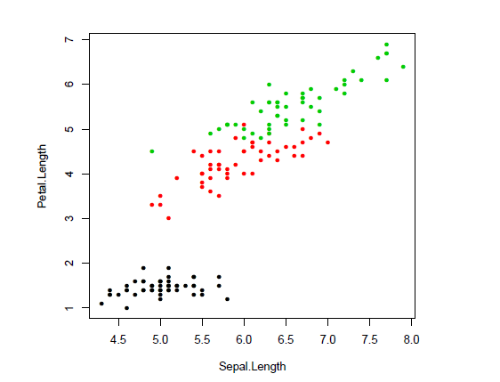
From the graph evidence of a strong correlation between the two measures is apparent, then we compute the correlation matrix of all numeric columns in dat, we round the results at the second decimal figure:
> ### correlation
> round(cor(dat[,-5]),2)
| Sepal.Length | Sepal.Width | Petal.Length | Petal.Width | |
| Sepal.Length | 1.00 | -0.12 | 0.87 | 0.82 |
| Sepal.Width | -0.12 | 1.00 | -0.43 | -0.37 |
| Petal.Length | 0.87 | -0.43 | 1.00 | 0.96 |
| Petal.Width | 0.82 | -0.37 | 0.96 | 1.00 |
The function text can be used to add the correlation value to the plot.
> plot(dat[,1],dat[,3],pch=20,xlab=colnames(dat)[1],ylab=colnames(dat)[3],col=dat[,5])
> text(4.5,6.2,paste("corr.",round(cor(dat[,1],dat[,3]),2)))
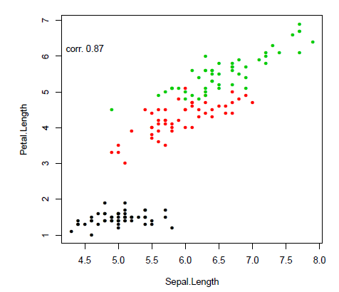
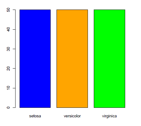
The function paste concatenates strings (to see all its options type ?paste). To obtain information on categorical quantities we need their frequency distributions, that is obtained by typing: table(dat$Species) Graphical representations for frequency distributions are the barplot and the pie chart:
> barplot(table(dat$Species),col=c("blue","orange","green"))
> pie(table(dat$Species))
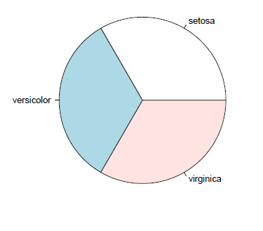
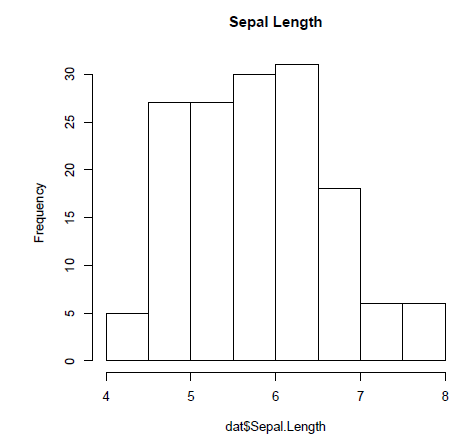
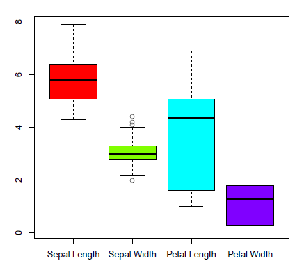
Relevant representations for numeric variables are histograms and boxplots:
> hist(dat$Sepal.Length,main="Sepal Length")
> boxplot(dat[,-5],col=rainbow(4))
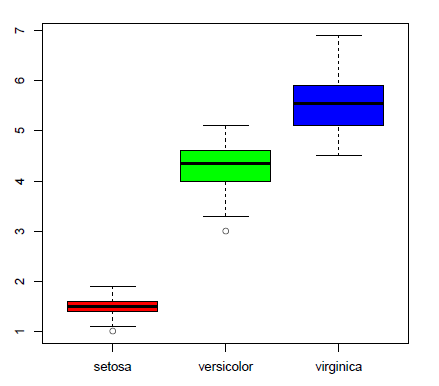
boxplot of one numeric variable with groups defined by a categorical factor
> boxplot(dat$Petal.Length~dat$Species,col=rainbow(3))
A large part of statistical procedures rely on the assumption that data are Gaussian. A simple graphical way to verify this assumption is trough quantile plots where empirical quantiles are compared to the standard normal theoretical quantiles (qq-plots).
> qqnorm(scale(dat$Sepal.Length))
> abline(c(0,1),col=2)
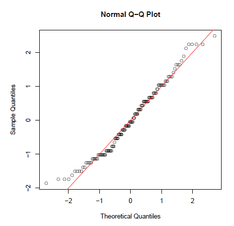
if points are close to the red line (the quadrant bisecting line) the normality assumption is acceptable.
The first R session is over. It is then possible to save all created objects using
> save.image("finalfirstsession.RData")
To remove all objects clearing the workspace type
> rm(list=ls())
Alcuni grafici semplici
Per realizzare un grafo a dispersione della prima e terza colonna del dataframe dat con colori diversi per specie, digitare:
> plot(dat[,1],dat[,3],pch=20,xlab=colnames(dat)[1],ylab=colnames(dat)[3],col=dat[,5])
Dal grafico si evince una forte correlazione fra le due misure, quindi si calcola la matrice di correlazione di tutte le colonne numeriche in dat, si arrotondano i risultati alla seconda cifra decimale:
> ### correlazione
> round(cor(dat[,-5]),2)
| Sepal.Length | Sepal.Width | Petal.Length | Petal.Width | |
| Sepal.Length | 1.00 | -0.12 | 0.87 | 0.82 |
| Sepal.Width | -0.12 | 1.00 | -0.43 | -0.37 |
| Petal.Length | 0.87 | -0.43 | 1.00 | 0.96 |
| Petal.Width | 0.82 | -0.37 | 0.96 | 1.00 |
La funzione text() puó essere usata per aggiungere il valore di correlazione sul grafico.
> plot(dat[,1],dat[,3],pch=20,xlab=colnames(dat)[1],ylab=colnames(dat)[3],col=dat[,5])
> text(4.5,6.2,paste("corr.",round(cor(dat[,1],dat[,3]),2)))
La funzione paste() concatena stringa (per vedere tutte le sue opzioni digitare ?paste). Per avere informazioni sulle quantitá categoriche si ha bisogno delle loro distribuzioni di frequenza, ottenuto digitando: table(dat$Species)
Le rappresentazioni grafiche delle distribuzioni di frequenza sono i grafici a barre o a torta:
> barplot(table(dat$Species),col=c("blue","orange","green"))
> pie(table(dat$Species))
Importanti rappresentazioni per variabili numeriche sono gli istogrammi e i boxplot:
> hist(dat$Sepal.Length,main="Sepal Length")
> boxplot(dat[,-5],col=rainbow(4))
boxplot di una variabile numerica con gruppi definiti da un fattore di categoria
> boxplot(dat$Petal.Length~dat$Species,col=rainbow(3))
Una grande parte delle procedure statistiche si basano sull'assunzione che i dati sono gaussiani. Un semplice modo grafico per verificare quasta assunzione é attraverso i i grafici di quantili, dove quantili empirici sono confrontati con i quantili teorici normali (qq-plots).
> qqnorm(scale(dat$Sepal.Length))
> abline(c(0,1),col=2)
se i punti sono vicini alla linea rossa (la linea bisettrice del quadrante), l'assunzione di normalitá é accettabile.
Terminata la prima sessione di R, é possibile salvare tutti gli oggetti creati con
> save.image("finalfirstsession.RData")
Per eliminare tutti gli oggetti e pulire lo spazio di lavoro, digitare:
> rm(list=ls())
Final Tips
Few rules to be kept in mind in order to avoid chaos:
- Keep your initial workspace empty - no objects
- Import the raw data and perform the analyses. Remember: a data file must be as simple as possible, just column header, data organized so that each row is a case
- From the File menu, or using the line command save the workspace in a project folder with a name of your choice (but with an extension of .RData).
- Get into the habit of keeping good clean code in your script file and save that in the project folder as well.
- By working keeping separate workspaces, all data objects and analysis objects will be available for subsequent analyses and there will be no need to import the data more than once.
Suggerimenti finali
Alcune regole da tenere a mente per evitare caos:
- Tenere lo spazio di lavoro iniziale vuoto - nessun oggetto
- Importare dati "grezzi" ed eseguire le analisi. Ricordarsi: il file dati dev'essere il piú semplice possibile, solo intestazioni di colonna e i dati devono essere organizzati in modo tale che ogni rigo é un caso
- Dal menu "File", o utilizzando la riga di comando salvare lo spazio di lavoro in una cartella di progetto con un nome a scelta (ma con l'estensione .RData).
- É buona abitudine mantenere il codice pulito negli script e salvare anche lo script nella cartella del progetto.
- Nel lavoro tenere spazi di lavoro separati, tutti gli oggetti di dati e gli oggetti di analisi saranno disponibili per successive analisi e non sará necessario importare di nuovo i dati.