The Incidence Function Model - Part I
| Site: | LifeWatch ERIC Training Platform |
| Course: | Spatially explicit metapopulation model - Incidence Function Model |
| Book: | The Incidence Function Model - Part I |
| Printed by: | Guest user |
| Date: | Tuesday, 15 September 2026, 2:26 PM |
Description
The basic Incidence Function model and its modifications will be here presented following Hanski (1994), H94 hereafter. The practical and theoretical differences about the models will be discussed here and in Units 9-11.
1. The Basic Model
We consider an assemblage of n patches composed of favorable habits for a given species, as in Figure 1.2. This assemblage is able to sustain a system of at most n local populations connected through exchange of individuals to build a metapopulation. It is assumed that the local dynamics, i.e. changes in the sizes of local populations, occur fast in comparison with metapopulation dynamics, colonization of currently empty habitat patches (H94).
In the IFM, at discrete time (years), the presence or absence (occupancy) of the species at any patch i is described by a first-order, homogeneous Markov chain with two states (0, 1) (empty and occupied, respectively). Let Pi the transition matrix describing the dynamics at site i
|
Pi |
0 |
1 |
|
0 |
1- Ci |
Ci |
|
1 |
Ei |
1- Ei |
where Ei := Pi(1, 0) and Ci := Pi(0, 1) are the extinction and colonization probabilities, respectively. The cases Ei = Ci = 0 and Ei = Ci = 1 are always excluded. The stationary distribution \(\pi\)i* then exists (see Eq. (3.5)) and, as in H94, we will use the notation
(4.1)\(J_i=\pi_i^* (1)= \frac{C_i}{C_i+E_i}\)The probability Ji is called incidence. Thanks to both the ecological assumptions and the Asymptotic results of Unit 3, it is assumed that the occupancy process at site i has reached its equilibrium state. In ecological terms, Ji represents the model-predicted long-term probability of patch occupancy.
The probabilities Ei and Ci are calculated independently for each patch i and are assumed do not depend on time. These probabilities are defined by referring to environmental and biological variables and to the life-history traits of the species.
The extinction probability depends on the patch area:
|
(4.2) |
Ei |
= |
(A0 / Ai ) x |
if Ai > A0 |
||||||||||||
|
|
|
|
|
|||||||||||||
|
Ei |
= |
1 |
if Ai ≤ A0 |
where A0 > 0 is the critical patch area for which the local population has a unity probability of extinction in 1 year and x > 0 reflects the severity of environmental stochasticity (H94).
Remark 4.1. In H94 a different notation is used: = e, where e is a positive constant. This has some consequences on parameter estimation, but this issue will not be discussed in this course. The interested people can also refer to Moilanen (1999).
Let be A0 = 1. For three different values of the patch area A (1.25, 2, 3.3), the effect of the parameter x is illustrated in Figure 4.1: the higher the value of x the lower the extinction probability, as expected from (4.2). The picture highlights, for a fixed value of x, that extinction probabilities quickly become very small for slowly increasing patch area (w.r.t. A0. Please, note that having settled A0 = 1, the three values of A correspond to the ratio of A to A0) .
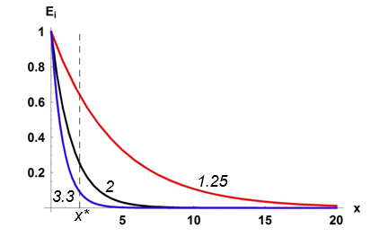
Figure 4.1 - Effect of habitat stochasticity values x for different values of Ai (/A0). The dashed vertical line highlights that for a fixed value x* of x, the extinction probability decreases with increasing Ai (/A0).
The colonization probability is a function of the number of immigrants arriving at patch i per year, Mi (H94). Under the assumption that the year-to-year variation of this number is negligible, in the IFM the colonization probability increases from 0 to 1 with increasing numbers of immigrants.
(4.3)\(C_i=\frac{M_i^2}{M_i^2+y^2 }\)where y > 0 describes the colonization ability of the species (H94).
For three different values of Mi, (10, 30 and 100) the effect of the parameter y is illustrated in Figure 4.2: the higher the value of y the lower the colonization probability. For a fixed value of y, the colonization probability approaches unity with increasing Mi.
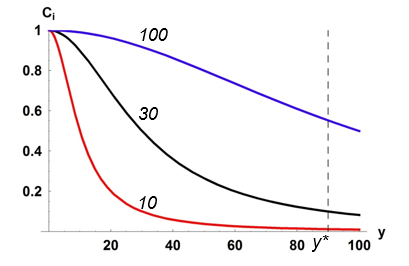
Figure 4.2 - Effects of parameter y on the colonization probability for three different values of Mi. The dashed vertical line highlights that for a fixed value y* of y, the colonization probability increases with increasing Mi.
As the estimation of Miis a difficult task, in the IFM the immigration numbers are assumed to be proportional to connectivity Si :
(4.4)\(M_i=\beta S_i=\beta \sum_{(k≠i)}\delta_i exp{(-\alpha d_{ik})}A_k\)where δi is the observed incidence of the site i, \(\alpha\) is a positive constant setting the survival rate of migrants over the distance, dik the centroid-to-centroid distance between patches i and k. Then, the colonization probability can be re-written as
(4.5)\(C_i=\frac{S_i^2}{S_i^2+y^2}\)where now y is used in place of y/β (in H94 y/β is denoted by y').
Example 4.1.We will use the free software R (R Core Team 2014) to analyze simulated metapopulation data. This software can be installed from the webpage http://cran.r-project.org/.[1]
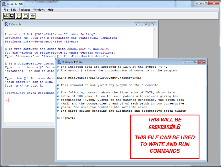
Window users can launch R by clicking on the shortcut on their Desktop. A window like this
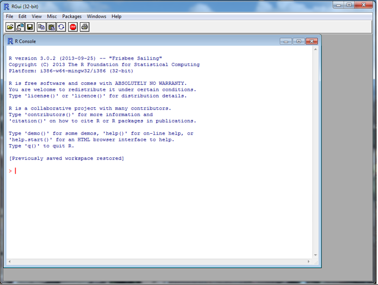
will appear, where the symbol " > | " (the prompt) indicates where you will type the commands. The output (if any) will be displayed after each command on the R console.
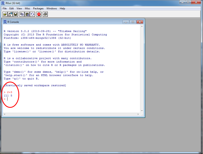
An alternative and very convenient way to run a list of commands, and to write and then run a program, is to use a script file. Let IFMcourse be a new directory on your computer that will be the working directory for this course. Select "New script" from the "File" menu and save the file as the commands.R file in IFMcourse. Then, from the "File" menu this directory can be selected as working directory by the option "Change directory". Copy on commands.R all the R instructions will be given and then run each command as it is introduced by selecting the corresponding line (simply, put the prompt "|" on the selected command line) and by typing CTR+R . The selected command will appear on the R console, together with the output, if any.
Linux users can find analogous user interfaces, like “rstudio” (http://www.rstudio.com/ ).
To start this example, download the file REFMETAPOP.txt in the directory IFMcourse. This file contains data about a reference metapopulation of 100 patches in an area of 50 Km x 50 Km. This metapopulation will be used in almost all the examples of this course.
To read the file REFMETAPOP.txt and create a data frame from it, with patches corresponding to lines and variables to fields in the file, we use the command read.table. For more information on this command (and on any other command):
help(read.table)
Any R instruction or comment will be given in a different font. These instructions and comments can be directly copied on either the R console or the file commands.R. Sometime, partial or complete R output is provided as it appears in the R console, typed in light black.
[1] Please, note that this is not a course on R: in this course, the necessary R commands to understand how the IFM works will be introduced and described. People interested on the R language can refer to http://www.r-project.org/doc/bib/R-books.html for a wide bibliography.
# The imported data are assigned to DATA by the symbol "<-".
# The symbol # allows the introduction of comments in the program.
DATA<-read.table("REFMETAPOP.txt",header=TRUE)
# This command does not yield any output on the R console.
#
# The following command shows the first rows of DATA, which is a
# table of 100 rows (1 row for each patch) with columns giving the
# coordinates (x.crd, y.crd) of the patches centroids, the patch area
# (Km2) and the occupancies p and p1 of each patch in two consecutive
# years. One more row contains the variable names.
# The first column contains the automatic and progressive patch number
head(DATA)
x.crd y.crd A p p1
1 46590.46 36459.168 0.1136916 0 1
2 38249.50 10209.727 1.4513826 1 0
3 16391.89 5495.438 0.1097466 0 1
4 31459.17 29865.312 0.4003912 1 0
5 45574.37 21531.567 0.5048622 1 0
6 34341.12 18033.422 1.5203295 1 0
# As DATA is a matrix, the data of the 13-th patch is
DATA[13,]
x.crd y.crd A p p1
13 29873.62 29428.68 1.437852 1 0
# while the content of the second column (y.crd) is
DATA[,2]
[1] 36459.168 10209.727 5495.438 29865.312 21531.567 18033.422 7068.673
[8] 33847.654 4647.137 15675.847 17288.728 5109.739 29428.677 32837.209
[15] 20720.949 34522.399 31119.758 15466.859 9908.575 41754.838 26569.624
[22] 33722.895 26085.585 23839.249 43304.326 26208.987 40887.537 19894.654
[29] 11318.515 39315.309 37144.766 40417.921 12973.940 33006.967 44749.996
[36] 23853.809 29064.176 1950.972 39739.414 39771.907 20208.517 6202.474
[43] 22052.480 20933.666 9141.167 10674.119 22612.318 6626.768 30078.350
[50] 26246.577 42278.952 3846.805 30810.778 31978.060 6726.060 27927.268
[57] 24078.376 36027.738 31035.589 25136.793 25083.867 2557.595 8696.669
[64] 22756.651 32102.562 24475.929 21551.672 8476.308 16450.155 38489.949
[71] 3786.379 33921.527 28166.911 17184.357 30022.402 43374.797 30169.833
[78] 1160.344 40887.241 19464.682 40284.146 23481.162 11302.356 22750.429
[85] 8117.678 40156.075 3115.955 7947.082 37069.232 19747.159 33886.554
[92] 17988.140 2119.424 32477.187 32092.176 30309.681 34562.133 5785.241
[99] 32327.827 43427.543
# The occupancy of the 87-th patch at the first year is
DATA[87,4]
[1] 0
# The following command allows the use of the variable's names
attach(DATA)
# so that the occupancy of the 87-th patch at the first year is also
p[87]
[1] 0
# By the following command the main descriptive information about each
# variable is provided.
summary(DATA)
x.crd y.crd A p p1
Min.:250.8 Min.:1160 Min.:0.07329 Min.:0.00 Min.:0.00
1st Qu.:19260.9 1st Qu.:12560 1st Qu.:0.31858 1st Qu.:0.00 1st Qu.:0.00
Median:28155.6 Median:24780 Median :0.80927 Median :0.00 Median :1.00
Mean:26923.4 Mean:23772 Mean:1.25765 Mean:0.45 Mean:0.61
3rd Qu.:37106.1 3rd Qu.:33186 3rd Qu.:1.53142 3rd Qu.:1.00 3rd Qu.:1.00
Max.:49635.7 Max.:44750 Max.:8.14282 Max.:1.00 Max.:1.00
# How many patches were occupied at the first year is
sum(p)
[1] 45
# The commons statistical plots histogram and boxplot are obtained by
# the commands “hist” and “boxplot”, here applied to the patch areas
hist(A)
# and
boxplot(A)
# Note that plots are displayed in a separate window (R Graphics)which
# activates a different menu bar.
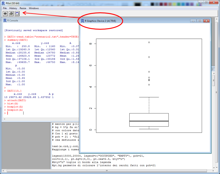
# Plots can be saved in different formats (File menu). Note also that
# a new plot deletes the previous one: explore the History menu to
# fix this issue.
# In the rest of this example we will refer to the vector p only.
# By the following command we obtain the usual representation, like in # Figure 1.2, of the metapopulation
plot(x.crd,y.crd,asp=1,xlab="",ylab="",cex=sqrt(A*3),pch=21,col=p+1,bg=5*p,main="REFERENCE METAPOPULATION")
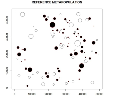
# col=p+1 (col=colors) yields the black border to circles,
# representing empty patches (p[i]=0); while occupied patches (p[i]=1)
# have a red border (almost invisible in the previous picture).
# By xlab="",ylab="" it is possible to label the axes.
# bg = 2*p yields a colored disk for occupied patches (p[i] = 1, 1=black, # 2=red, and so on), and a white disk (bg = 0) for empty patches.
# pch = 21 yields a "filled circle" as patch shape.
# cex defines the size of the disks, here proportional to A
# By main=" " it is possible to give a title to the picture.
#
# By
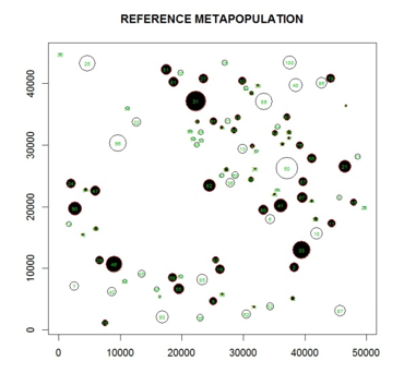
text(x.crd,y.crd,labels=c(1:100),cex=0.5,col=2)
# the identifying patch numbers can be added to the plot.
# c(1:100) means the vector of the integer numbers from 1 to 100.
# To close the R console, use the command
q()
# Users who used the script to run the commands, can answer NO to the
# pop-up question “Save the workspace image?”, as commands and
# definitions are directly saved on the script file. Users who
# directly ran the commands on the R console might answer YES: this# allows to save all commands and definitions, which can be retrieved
# by the up arrow key (-) at the next launch of R.
2. The Basic Model - References
Moilanen A. (1999) - Patch occupancy models of metapopulation dynamics: efficient parameter estimation using implicit statistical inference. Ecology 80,1031–1043.
R Core Team (2014). R: A language and environment for statistical computing. R Foundation for Statistical Computing, Vienna, Austria. URL http://www.R-project.org/.