A few hints about the ecological problem and the Incidence Function Model (IMF)
| Site: | LifeWatch ERIC Training Platform |
| Course: | Spatially explicit metapopulation model - Incidence Function Model |
| Book: | A few hints about the ecological problem and the Incidence Function Model (IMF) |
| Printed by: | Guest user |
| Date: | Tuesday, 15 September 2026, 2:26 PM |
Description
A few hints about the ecological problem and the Incidence Function Model
Overview
This Unit is essentially based on the papers by Gilioli et al. (2008), Bodini et al. (2008), Gilioli et al. (2013) and on a few talks given by the present author. Any omissions or errors should be ascribed to the present author only (a mathematician, not an ecologist).
A few hints about the ecological problem and the Incidence Function Model (IFM)
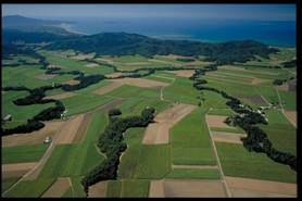
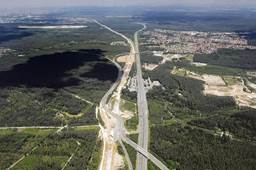
Habitat fragmentation, reduction and degradation as well as the quality of habitat connecting environments are critical for species persistence.
 |  |
 | 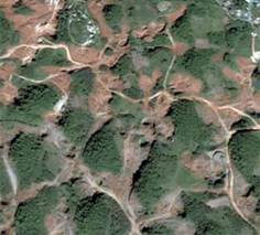 |
Figure 1 – Some examples of habitat fragmentation.
A few hints about the ecological problem and the Incidence Function Model (IFM) - Page 1/6
The concept of habitat fragmentation has been deeply discussed, for instance, in Franklin et al. (2002) and in Didham (2010).
In fragmented landscapes, populations are often structured as a
metapopulation (Melbourne et al., 2004), that is as a
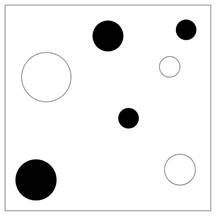
set of local populations within some larger area, where typically migration from one local population to at least some other patches is possible (Hanski and Simberloff, 1997). Figure 2 represents by a diagram a small metapopulation with four occupied patches (the black disks) and three empty patches (the circles).
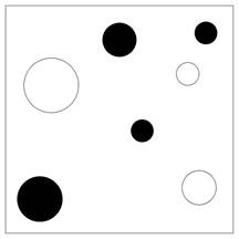 |
| Figure 2 - Diagram of a small metapopulation. Black disks: occupied patches; circles: empty patches. Migrations from occupied to empty patches are possible. |
Metapopulation models were originally proposed for pests and were based on a simple description of the frequency of occupied patches (Levins, 1969; Ives and Settle, 1997).
 |
|
| Figure 3 – Prof. Richard Levins and the Levins model. |
In the Levins model (Figure 3) it is assumed that all the habitat patches are similar, so that according to this model, a diagram of the spatial structure of a metapopulation should be as in Figure 4, where all the patches are represented by equal and contiguous squares, so that the spatial information disappears.
 |
| Figure 4 – Metapopulation spatial structure for Levins-type models: patches are represented by equal and contiguous squares. |
A few hints about the ecological problem and the Incidence Function Model (IFM) - Page 2/6
In general, the objects for conservation are populations, and predictions as well as ranking of management strategies are based on demographic approaches and viability analyses (Akçakaya & Sjögren-Gulve, 2000; Drechsler & Burgman, 2004). With respect to conservation biology, the main question is whether a given species is likely to persist as a metapopulation in a particular set of habitat patches, and how modifications in the number, quality and connectivity of habitat patches may affect population viability (Hanski, 1999). These aspects are even more important when conservation strategies have to be implemented in areas with intensified agriculture, residential zones or industrial sites, where they could give rise to conflicts of interest among different land users.
The clear need for an explicit representation of patches in space has demanded the development of different metapopulation models. In this course, Figure 2 or similar pictures will be used to represent a metapopulation as described by a spatially explicit metapopulation model. Unlike Figure 4, such pictures allow us to visualize the differences among patch areas and between-patches distances, for instance, two key elements of the metapopulation spatial structure. Figure 2, however, differs from a third kind of spatial representation, like that in Figure 5, typical of landscape analysis. In this case, the geographical information reaches a higher level of detail, often coming from a spatial analysis by a GIS software.
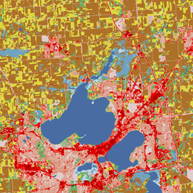 |
| Figure 5 – Land cover surrounding Madison, WI. Fields are colored yellow and brown, water is colored blue, and urban surfaces are colored red. |
A few hints about the ecological problem and the Incidence Function Model (IFM) - Page 3/6

Prof. Ilkka Hanski (University of Helsinki) |
Twenty years after the seminal paper of Ilkka Hanski A practical model of metapopulation dynamics (Hanski, 1994), introducing the Incidence Function Model (IFM) as a spatially explicit stochastic model for metapopulation dynamics, the statement about the lack of analytical models of metapopulation dynamics able to incorporate specific information about patch locations and hence able to generate predictions about specific metapopulations still holds true. Despite some criticism (Baguette 2004), this makes the Incidence Function Model and its extensions noteworthy for ecological applications. The web site of the Metapopulation Research Group of Helsinki (http://www.helsinki.fi/science/metapop/index.htm) provides a wide panorama of a relevant part of recent researches on “the biology of species inhabiting fragmented landscape”, aiming also at applying “the core concepts of metapopulation biology to management and conservation of landscapes and biodiversity”. |
|
The IFM is based on four elements: 1. presence/absence data 2. patches locations 3. areas (including patch quality) 4. intra-patches distances (including matrix quality). This model does not consider the particular patch shape: all these issues justify the choice of pictures like Figure 2 (where all the patches are circular) to represent a metapopulation in this course. |
 |
A few hints about the ecological problem and the Incidence Function Model (IFM) - Page 4/6
The IFM relates the extinction probability of a patch to its area: the larger the patch the lower the extinction probability, as indicated in Figure 6 by different thickness of the red arrows.
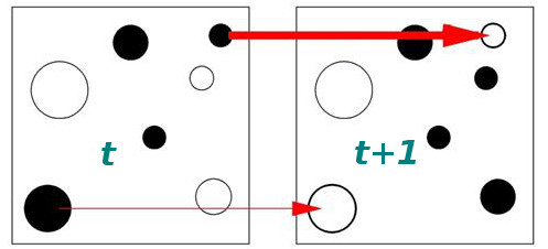
Figure 6 – At time t +1, any occupied patch could go extinct. The larger the patch the lower the extinction probability: in this picture this fact is marked by the different thickness of the arrows of two extinct populations: the thicker the red arrow, the higher the extinction probability.
A few hints about the ecological problem and the Incidence Function Model (IFM) - Page 5/6
The colonization probability of any patch depends on the contribution from all the other occupied patches. In Figure 7, all the patches occupied at time t contribute to the colonization of patch A at the following time, t+1, as indicated by the red arrows. Each contribution depends on both the patch area (the larger the area, the higher the contribution) and the distance from patch A (the longer the distance, the lower the contribution). That is, the colonization probability depends on the connectivity of the patch.
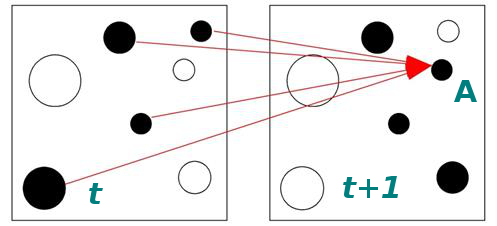
Figure 7 - At time t +1, any empty patch could become occupied by colonization. All the occupied patches give a contribution to the colonization of patch A, according to both their area and distance from A.
In other words, in the IFM the patch area is assumed as a proxy for the population size, while the intra-patches distance takes into account the survival rate of migrant over the distance.
A few hints about the ecological problem and the Incidence Function Model (IFM) - Page 6/6
Spatially explicit metapopulation models are a widely used tool in conservation biology (Vos et al. 2000, Ter Braak & Etienne 2003; Gilioli et al. 2008), while they have received little attention in pest control (Hunter 2002; Gilioli et al. 2013). The apparent lack of interest in applying the IFM and its generalizations to pest is surprising, because it would enable managers to take into account several spatial and habitat features (Gilioli et al. 2013), and express management actions as far as management outcomes in terms of model variables.
Indeed, variations in patches locations could be considered for management (Figure 8b), as well as variations in some patches areas (Figure 8c) and patch occupancies (Figure 8d) for instance.
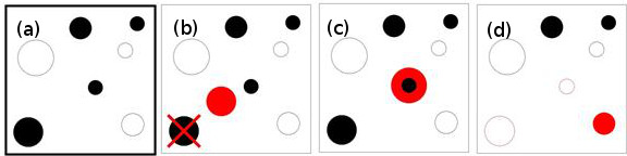
Figure 8 – Instances of management actions represented by changes to model variables, compared to the original metapopulation (a). (b) Variation of a patch location (from the crossed black to the red one); (c) variation of patch area (from black to red); (d) variation of patch occupancy of the red circles/disks.
This is particularly relevant for management. Indeed, in the most recent years it has been pointed out that metapopulation models should be embedded in a decision-making framework to give managers the capability of ranking alternative decisions (Westphal et al., 2003). This means that the objectives of the management should be explicitly and clearly stated in terms of metapopulation model variables (Possingham et al., 2001; Gilioli et al. 2013), to also underpin an efficient allocation of resources.
Final remark
For the sake of completeness, it should be pointed out that habitat fragmentation alone is not enough to define a metapopulation. Murphy et al. (1990) request small body size, high rate of population increase, short generation time and high habitat specificity. In order that a plant-pest system can be considered as a metapopulation, Hanski (1997) recommends that host plants are distributed as discrete patches, pest populations within patches have a substantial risk of extinction, empty patches are available for colonization, and pest local populations do not fluctuate synchronously. This topic will not be considered in this course.
References
Akçakaya H.R., Sjögren-Gulve P. (2000) - Population viability analysis in conservation planning: an overview. Ecological Bulletin, 48, 9–21.
Baguette M. (2004) - The classical metapopulation theory and the real, natural world: a critical appraisal. Basic and Applied Ecology, 5, 213-224.
Bodini A., Baumgaertner J., Gilioli G. (2008) - Conservation strategies evaluation in an adaptive management framework (commentary). Animal Conservation, 11, 472-475
Didham R. K. (2010) - Ecological Consequences of Habitat Fragmentation. In: eLS. John Wiley & Sons, Ltd., Chichester. DOI: 10.1002/9780470015902.a0021904.
Drechsler M., Burgman M. (2004) - Combining population viability analysis with decision analysis. Biodiversity Conservation, 13, 115–139.
Franklin A.B, Noon B.R., George T.L. (2002) – What is habitat fragmentation? Studies in Avian Biology, 25, 20-29.
Gilioli G., Bodini A., Baumgaertner J., Weidmann P., Hartmann J. (2008) - A novel approach based on Information Theory to rank conservation strategies: an application to amphibian metapopulations (with discussion). Animal Conservation, 11, 453-462
Gilioli G., Bodini A., Baumgaertner J. (2013) - Metapopulation modelling and area-wide pest management strategies evaluation. An application to Pine processionary moth. Ecological Modelling, 260, 1-10.
Hanski I. (1994) - A practical model of metapopulation dynamics. Journal of Animal Ecology, 63, 151-162.
Hanski I. (1997) - Metapopulation dynamics: from concepts and observations to predictive models. In: Hanski I. & Gilpin M.E. (eds.), Metapopulation Biology: Ecology, Genetics and Evolution. Academic Press, San Diego, USA, 69–91.
Hanski, I. (1999). Metapopulation ecology. Oxford: Oxford University Press.
Hanski I., Simberloff D. (1997) - The metapopulation approach, its history, conceptual domain and application to conservation. In: Hanski I. & Gilpin M.E. (eds.), Metapopulation Biology: Ecology, Genetics, and Evolution. Academic Press, San Diego, USA, 5-26.
Hunter M.D. (2002) - Landscape structure, habitat fragmentation, and the ecology of insects. Agricultural and Forest Entomology 4, 159–166.
Ives A.R., Settle W.H. (1997) - Metapopulation dynamics and pest control in agricultural systems. American Naturalist 149, 220-246.
Levins R. (1969) - Some demographic and genetic consequences of environmental heterogeneity for biological control. Bulletin of the Entomological Society of America, 15, 237-240.
Melbourne B.A., Davies K.F., Margules C.R., Lindenmayer D.B., Saunders D.A., Wissel C., Henle K. (2004) - Species survival in fragmented landscapes: where to from here. Biodiversity Conservation, 13, 275–284.
Murphy D.D., Fraes K.E., Weiss S.B. (1990) – An environment-metapopulation approach to viability analysis for a threatened invertebrate. Conservation Biology, 4, 41–51
Possingham H.P., Andelman S.J., Noon B.R., Trombulak S., Pulliam H.R. (2001) - Making smart conservation decisions. In: Soule M.E. & Orians G.H. (Eds.), Conservation Biology: Research Priorities for the Next Decade. Pulliam Press, Washington, USA, 225–244.
Ter Braak C.J, Etienne R.S. (2003) - Improved Bayesian analysis of metapopulation data with an application to a tree frog metapopulation. Ecology, 84, 231-241.
Vos C.C., ter Braak C.J.F., Nieuwenhuizen W. (2000) - Incidence Function modelling and conservation of the tree frog Hyla arborea in the Netherlands. Ecological Bulletin, 48, 165-180.
Westphal M.I., Pickett M., Getz W.M., Possingham H.P. (2003) - The use of stochastic dynamic programming in optimal landscape reconstruction for metapopulations. Ecological Applications, 13, 543-555.