About this Tutorial
| Site: | LifeWatch ERIC Training Platform |
| Course: | Species Distribution Modelling (SDM): A Guide |
| Book: | About this Tutorial |
| Printed by: | Guest user |
| Date: | Tuesday, 15 September 2026, 2:35 PM |
Description
A brief description of rationale, aim and structure of the tutorial.
Overview
- Introduction to Species Distribution modelling: aim, theory, applications
- Aim and Scope
- Contents and Structure
- Preparatory materials, software and data
Species Distribution Modeling: aims, theory and applications
In the last decade Species Distribution Modelling (SDM) become a technique widely used in many fields of natural and biological sciences to infer the ecological requirements of species and to predict their geographic distributions (Elith & Leathwick, 2009). Species distribution models can be used to support conservation decision making (Guisan et al., 2013). Forecasting endangered species distribution under climatic change scenario is increasingly used in conservation biology (Muñoz et al., 2013), while forecast the spread of invasive species is receiving a growing interest in invasion biology (Verbruggen et al., 2013). Furthermore, many phylogeographic studies, focusing on the influence of past climatic changes on the observed spatial distribution of genetic diversity, merge information from molecular biology and SDM to infer intra-specific evolutionary patterns (Knowles et al., 2007; Alvarado-Serrano & Knowles, 2014). Species distribution models are also known as ecological niche models (ENM), habitat suitability models and bioclimatic envelope modelling. Many researchers consider these definitions mainly as synonyms and here we will refer to this class of methods as SDM. However, it worth to note that some others researchers pointed on the fact that these terms (particularly SDM and ENM) are not fully interchangeable and their differences are not merely semantic (Townsend Peterson, 2006; Townsend Peterson & Soberón, 2012) but depend of the choice of the set of variables used to predict niche and distribution and to the focus of the study (i.e. niche quantification versus spatial predictions). From a practical point of view, both SDM and ENM are identical: use the same software, largely rely on similar assumptions and in most of the cases share the same set of predictors. The aim of SDMs is to infer the probability of occurrence of a taxon given a set of variables (climate, elevation, soil type, etc.) that are assumed to be related to the distribution and habitat preferences of the taxon under study. The habitat suitability of a give species is then extrapolated on the basis of the conditions observed in known occurrence sites (Fig. 1). The inference of habitat suitability and distribution range of a species might be accomplished by using different algorithms (see below). This wide array of statistical approaches offers flexibility and can address different problems. However, the quality and reliability of SDMs depends always on the quality and appropriateness of the species occurrences and environmental data inputs, the expert opinion and the recognition and treatment of uncertainty in the model outputs.
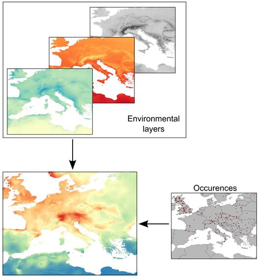
Figure 1: A scheme of Species Distribution Model. Environmental layers (climate, elevation, soil types) combined with known occurrences allow to identify the potential distribution of a species
Aim and Scope
This tutorial does not pretend to be an exhaustive guide on species distribution models. It wants to provide some practical advices on how to perform first basis steps to students and researchers that are not familiar with SDM. The tutorial is not intended as a treaty of statistics and modelling. Readers should be already familiar with the R statistical environment, have some basic knowledge of statistics and be familiar with ecology theory needed for a correct design of the analysis and its interpretation. The example of SDM provided by this tutorial is relatively simple (if you are familiar with R) and it should be not difficult to apply the same workflow to your own data.
Contents and Structure
The tutorial is composed in 5 modules:
1. Occurrence data
2. The environmental variables
3. Running the analysis
4. The output interpretation and test of robustness
5. Survey of available software
In each of these sections we will provide practical examples on how to perform preliminary analyses, in order to minimize errors and to maximize to reliability of the results. Successively, we will show how to fit the models with different algorithms, or with a combination of these, and how to interpret correctly the results with aim of robustness test.
Preparatory materials, software and data
All the software, occurrences data and environmental layers used in this tutorial are freely available on the web. To successfully complete the tutorial it is necessary to install on you computer the R statistic environment (http://www.r-project.org), the package dismo (http://cran.r-project.org/web/packages/dismo/index.html) and the package biomod2 (http://cran.r-project.org/web/packages/biomod2/index.html). The examples provided will be based on occurrences of the rose-ringed parakeet Psittacula krameri obtained from GBIF database. Environmental layers will be obtained from the Worldclim database (http://www.worldclim.org) . Some ready to use R scripts, created ad-hoc for the preparation of occurrences and environmental layers will be provided. Furthermore, all the procedure described in the tutorial, will be provided as R script. Additional R libraries could be necessary and is good that they will be installed on your machine before to start with this tutorial: “raster”, “rgeos”, “rgdal”, “fmsb”, “sp”. The scripts have been tested on different platform and different version of R. If you are using the very last version of R (to date the 3.1.2) and you encounter some problem in downloading libraries such as “rgeos” we suggest to downgrade to R 3.0.3. We will provide a zip archive with the R script (named “Tutorial.R”) necessary for all the modules of the tutorial, a folder (named “script”) containing additional R scripts, a folder (named “Shapefile_Pkrameri”) with the shapefile of the native range of P. krameri and the maxent jar file (version 3.3.3k downloaded from http://www.cs.princeton.edu/%7Eschapire/maxent/). All these files and folders must be placed in the same folder. Furthermore, it is necessary to download climatic layers for future condition from http://biogeo.ucdavis.edu/data/climate/cmip5/2_5m/cc85bi70.zip. The file included in this zip file must be extracted in a folder that must be named “future”. The newly created folder (and the climatic layers inside) must be placed in the same folder with the other files.
Alvarado-Serrano DF & Knowles LL. 2014. Ecological niche models in phylogeographic studies: applications, advances and precautions. Molecular Ecology Resources 14, 233–248
Elith, J. & Leathwick, J.R. 2009. Species distribution models: Ecological explanation and prediction across space and time. Annual Review of Ecology, Evolution, and Systematics 40: 677–697.
Guisan A, Tingley R, Baumgartner JB, Naujokaitis-Lewis I, Sutcliffe PR, Tulloch AI, Regan TJ, Brotons L, McDonald-Madden E, Mantyka-Pringle C et al. 2013. Predicting species distributions for conservation decisions. Ecology Letters 16(12) pp. 1424-1435
Knowles LL, Carstens BC, Keat ML. 2007. Coupling Genetic and Ecological-Niche Models to Examine How Past Population Distributions Contribute to Divergence. Current Biology
17: 940–946
Muñoz A-R, Márquez AL, Real R. 2013. Updating Known Distribution Models for Forecasting Climate Change Impact on Endangered Species. Plos ONE, 8: e65462.
Townsend Peterson A. 2006. Uses and requirements of ecological niche models and related distributional models. Biodiversity Informatics, 3: 59-72
Townsend Peterson A & Soberón J. 2012. Species Distribution Modeling and Ecological Niche Modeling: Getting the Concepts Right. Natureza & Conservação, 10:102-107.
Verbruggen H, Tyberghein L, Belton GS, Mineur F, Jueterbock A, Hoarau G, Gurgel GF, De Clerck O. 2013. Improving Transferability of Introduced Species’ Distribution Models: New Tools to Forecast the Spread of a Highly Invasive Seaweed. Plos ONE, 8: e68337.