Case study: the Po River Delta - Case study: il delta del fiume Po
The Po River Delta: Mixed effects models
We are interested in assessing which spatial scale (system, lagoon or monitoring station) seems more relevant in terms of representation of biodiversity variation. The fixed effects are given by the factors Vegetation and Sediment that describe the station environment. Being both explanatory variables categorical, their inclusion in the fixed part of the model implies that a fixed intercept for each combination of categories is estimated, plus the nested random effects of the the System and Lagoon factors. For comparison, we first consider a model with no explanatory variables, including only one fixed intercept and random intercepts ruled by the nested effects of System and Lagoon. Nested effects are represented using the syntax effect1/effect2/effect3....
> require(nlme)
> alpha.1=delta.part$CommunityAlphaEntropies
> sys=env$System
> lag=env$Lagoon
> mod0.delta=lme(alpha.1~1,random=~1|sys/lag,data=env,method="ML")
> summary(mod0.delta)
Linear mixed-effects model fit by maximum likelihood
Data: env
| AIC | BIC | logLik |
| 32.47187 | 37.01384 | -12.23593 |
Random effects:
Formula: ~1 | sys
(Intercept)
StdDev: 7.931876e-06
Formula: ~1 | lag %in% sys
(Intercept) Residual
StdDev: 0.2696757 0.3427638
Fixed effects: alpha.1 ~ 1
| Value | Std.Error | DF | t-value | p-value | |
| (Intercept) | 1.723163 | 0.1172432 | 13 | 14.69735 | 0 |
Standardized Within-Group Residuals:
| Min | Q1 | Med | Q3 | Max |
| -1.7897264 | -0.4813381 | 0.1724562 | 0.5263777 | 1.3500645 |
Number of Observations: 23
Number of Groups:
| sys | lag | %in% | sys |
| 3 | 10 |
We estimate the model including both explanatory variables: Vegetation and Sediment
> mod1.delta=lme(alpha.1~Vegetation+Sediment,random=~1|sys/lag,data=env,method="ML")
> summary(mod1.delta)
Linear mixed-effects model fit by maximum likelihood
Data: env
| AIC | BIC | logLik |
| 27.68141 | 36.76536 | -5.840703 |
Random effects: Formula: ~1 | sys
| (Intercept) | |
| StdDev: | 5.495947e-06 |
Formula: ~1 | lag %in% sys
| (Intercept) | Residual | |
| StdDev: | 1.127679e-06 | 0.3119242 |
Fixed effects: alpha.1 ~ Vegetation + Sediment
| Value | Std.Error | DF | t-value | p-value | |
| Intercept) | 1.4047387 | 0.1762978 | 11 | 7.967989 | 0.0000 |
| Vegetationmacroa | 0.7110108 | 0.2275994 | 11 | 3.123957 | 0.0097 |
| Vegetationnone | 0.4233437 | 0.2275994 | 11 | 1.860039 | 0.0898 |
| Vegetationsmacroph | -0.0252748 | 0.2493227 | 5 | -0.101374 | 0.9232 |
| Sedimentsand | 0.1286338 | 0.2493227 | 5 | 0.515933 | 0.6279 |
| Correlation: | |||||
| (Intr) | Vgttnm | Vgttnn | Vgttns | ||
| Vegetationmacroa | -0.775 | ||||
| Vegetationnone | -0.775 | 0.600 | |||
| Vegetationsmacroph | -0.707 | 0.548 | 0.548 | ||
| Sedimentsand | 0.000 | 0.000 | -0.365 | 0.000 |
Standardized Within-Group Residuals:
| Min | Q1 | Med | Q3 | Max |
| -2.5903194 | -0.5126984 | 0.1900709 | 0.6213941 | 1.9602155 |
Number of Observations: 23 Number of Groups:
| sys | lag | %in% | sys |
| 3 | 10 |
Notice that only some of the categories of Vegetation and Sediment are explicitly mentioned, this is called corner point parametrization, some reference categories are associated to the general intercept and the difference between these ones and the others are estimated. Then in the model summary of mod1.delta we have as corner point the combination of categories "emerged macrophytes" and "mud", while the other coeficients measure the difference with the corner point. The level "macroa" (presence of macroalgae) differs consistently from the corner point, some difference is also observed for the level "none", while the "sand" category of Sediment seems not to change significantly with respect to the corner point. We now try different models
> mod2.delta=lme(alpha.1~Vegetation,random=~1|sys/lag,data=env,method="ML")
> summary(mod2.delta)
Linear mixed-effects model fit by maximum likelihood Data: env
| AIC | BIC | logLik |
| 26.01904 | 33.9675 | -6.009521 |
Random effects: Formula: ~1 | sys
| (Intercept) | |
| StdDev: | 3.687605e-06 |
Formula: ~1 | lag %in% sys
| (Intercept) | Residual | |
| StdDev: | 8.330385e-07 | 0.3142222 |
Fixed effects: alpha.1 ~ Vegetation
| Value | Std.Error | DF | t-value | p-value | |
| (Intercept) | 1.4047387 | 0.1728598 | 11 | 8.126464 | 0.0000 |
| Vegetationmacroa | 0.7110108 | 0.2231610 | 11 | 3.186089 | 0.0087 |
| Vegetationnone | 0.4662216 | 0.2077516 | 11 | 2.244130 | 0.0464 |
| Vegetationsmacroph | -0.0252748 | 0.2444606 | 6 | -0.103390 | 0.9210 |
| Correlation: | |||||
| (Intr) | Vgttnm | Vgttnn | |||
| Vegetationmacroa | -0.775 | ||||
| Vegetationnone | -0.832 | 0.645 | |||
| Vegetationsmacroph | -0.707 | 0.548 | 0.588 |
Standardized Within-Group Residuals:
| Min | Q1 | Med | Q3 | Max |
| -2.7078336 | -0.3333537 | 0.1886809 | 0.5629413 | 1.9458803 |
Number of Observations: 23
Number of Groups:
| sys | lag | %in% | sys |
| 3 | 10 |
In the above summary it seems that the strongest differences in terms of fixed effects are found between stations with macroalgae and those without. Then we build a factor discriminating between presence/absence of macroalgae and we include again the factor Sediment into the model
> Macroa=ifelse(env$Vegetation=="macroa",1,0)
> Macroa=factor(Macroa)
> mod3.delta=lme(alpha.1~Macroa+Sediment,random=~1|sys/lag,data=env,method="ML")
> summary(mod3.delta)
Linear mixed-effects model fit by maximum likelihood Data: env
| AIC | BIC | logLik |
| 27.55772 | 34.37068 | -7.778858 |
Random effects: Formula: ~1 | sys
| (Intercept) | |
| StdDev: | 0.1882284 |
Formula: ~1 | lag %in% sys
| (Intercept) Residual | ||
| StdDev: | 9.551436e-06 | 0.3123423 |
Fixed effects: alpha.1 ~ Macroa + Sediment
| Value | Std.Error | DF | t-value | p-value | |
| (Intercept) | 1.5943983 | 0.1471106 | 12 | 10.838092 | 0.0000 |
| Macroa1 | 0.6161267 | 0.1777641 | 12 | 3.465978 | 0.0047 |
| Sedimentsand | 0.5193027 | 0.2310926 | 6 | 2.247162 | 0.0657 |
| Correlation: | |||||
| (Intr) | Macro1 | ||||
| Macroa1 | -0.304 | ||||
| Sedimentsand | -0.229 | 0.343 |
Standardized Within-Group Residuals:
| Min | Q1 | Med | Q3 | Max |
| -2.46104568 | -0.45583848 | -0.00266506 | 0.61053742 | 1.47064380 |
Number of Observations: 23
Number of Groups:
| sys | lag | %in% | sys |
| 3 | 10 |
To add a further term of comparison, we estimate the model with only the Macroa factor as fixed effect. Then we collect both AIC and BIC criteria and we chose the "best" model in statistical terms.
> mod4.delta=lme(alpha.1~Macroa,random=~1|sys/lag,data=env,method="ML")
> comp=data.frame(AIC=c(
+ AIC(mod0.delta),
+ AIC(mod1.delta),
+ AIC(mod2.delta),
+ AIC(mod3.delta),
+ AIC(mod4.delta)
+ ), BIC=c(
+ BIC(mod0.delta),
+ BIC(mod1.delta),
+ BIC(mod2.delta),
+ BIC(mod3.delta),
+ BIC(mod4.delta)
+ ))
> row.names(comp)=c("mod0","mod1","mod2","mod3","mod4")
> barplot(as.matrix(comp),beside=T,col=rainbow(5),legend=T,
+ args.legend=list(horiz=T,x="top",cex=0.7),ylim=c(0,45))
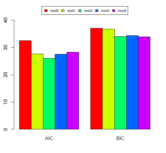
Model 2 is "the best", according to both AIC and BIC criteria. Mixed effects model comparison shows the general relevance of Vegetation and Sediment in determining the biodiversity variation. We now look again at the summary and verify if residuals of the chosen model are gaussian
> summary(mod2.delta)
Linear mixed-effects model fit by maximum likelihood Data: env
| AIC | BIC | logLik |
| 26.01904 | 33.9675 | -6.009521 |
Random effects: Formula: ~1 | sys
| (Intercept) | |
| StdDev: | 3.687605e-06 |
Formula: ~1 | lag %in% sys
| (Intercept) | Residual | |
| StdDev: | 8.330385e-07 | 0.3142222 |
Fixed effects: alpha.1 ~ Vegetation
| Value | Std.Error | DF | t-value | p-value | |
| (Intercept) | 1.4047387 | 0.1728598 | 11 | 8.126464 | 0.0000 |
| Vegetationmacroa | 0.7110108 | 0.2231610 | 11 | 3.186089 | 0.0087 |
| Vegetationnone | 0.4662216 | 0.2077516 | 11 | 2.244130 | 0.0464 |
| Vegetationsmacroph | -0.0252748 | 0.2444606 | 6 | -0.103390 | 0.9210 |
Correlation: |
|||||
| (Intr) | Vgttnm | Vgttnn | |||
| Vegetationmacroa | -0.775 | ||||
| Vegetationnone | -0.832 | 0.645 | |||
| Vegetationsmacroph | -0.707 | 0.548 | 0.588 |
Standardized Within-Group Residuals:
| Min | Q1 | Med | Q3 | Max |
| -2.7078336 | -0.3333537 | 0.1886809 | 0.5629413 | 1.9458803 |
Number of Observations: 23 Number of Groups:
| sys | lag | %in% | sys |
| 3 | 10 |
> qqnorm(residuals(mod2.delta))
> qqline(residuals(mod2.delta),col=2)
> shapiro.test(residuals(mod2.delta)) ### confirmed residuals are gaussian
Shapiro-Wilk normality test
data: residuals(mod2.delta)
W = 0.9383, p-value = 0.1651
To asses the random effects contribution to the alpha entropy measure, ob- serve the standard deviations given in the summary of the model
> ss=c(3.691927e-06,8.342304e-07)
> names(ss)=c("system","lagoon")
> barplot(ss,beside=T,col=c(5,3))
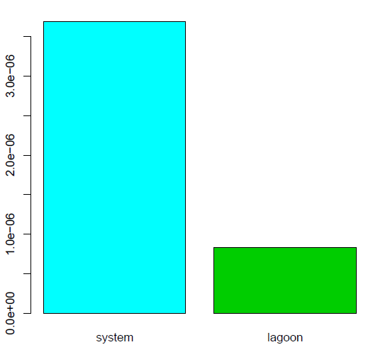
The graph above shows that the system level is the most relevant for these data. The use of mixed models facilitates the understanding of the spatial scale influence on biodiversity. Results emphasize that, in the Po river Delta, biodiversity conservation of lagoon ecosystems cannot be managed locally but, to be effective, requires a large scale process of governance.
Il delta del fiume Po: Modelli ad effetti misti (Mixed effects models)
Si è interessati alla determinazione quale scala spaziale (ecosistema, laguna o stazione di monitoraggio) sembra piú rilevante in termini di rappresentazione della variazione della biodiversitá. Gli effetti fissi sono dati dai fattori Vegetation (vegetazione) e Sediment (sedimento) che descrivono l'ambiente della stazione. Siccome sono variabili esplicative categoriche, la loro inclusione nella parte fissa del modello implica che verrá stimata un'intersezione fissa per ogni combinazione delle categorie, piú gli effetti casuali dei fattori System(sistema) e Lagoon (laguna). Per confronto, si considera un modello senza variabili esplicative, includendo solo una intersezione fissa e intersezioni casuali guidate dagli effetti annidati di System(sistema) e Lagoon (laguna). Effetti annidati sono rappresentati dalla sintassi effect1/effect2/effect3....
> require(nlme)
> alpha.1=delta.part$CommunityAlphaEntropies
> sys=env$System
> lag=env$Lagoon
> mod0.delta=lme(alpha.1~1,random=~1|sys/lag,data=env,method="ML")
> summary(mod0.delta)
Linear mixed-effects model fit by maximum likelihood
Data: env
| AIC | BIC | logLik |
| 32.47187 | 37.01384 | -12.23593 |
Random effects:
Formula: ~1 | sys
(Intercept)
StdDev: 7.931876e-06
Formula: ~1 | lag %in% sys
(Intercept) Residual
StdDev: 0.2696757 0.3427638
Fixed effects: alpha.1 ~ 1
| Value | Std.Error | DF | t-value | p-value | |
| (Intercept) | 1.723163 | 0.1172432 | 13 | 14.69735 | 0 |
Standardized Within-Group Residuals:
| Min | Q1 | Med | Q3 | Max |
| -1.7897264 | -0.4813381 | 0.1724562 | 0.5263777 | 1.3500645 |
Number of Observations: 23
Number of Groups:
| sys | lag | %in% | sys |
| 3 | 10 |
Si stima il modello includendo le due variabili esplicative: Vegetation e Sediment
> mod1.delta=lme(alpha.1~Vegetation+Sediment,random=~1|sys/lag,data=env,method="ML")
> summary(mod1.delta)
Linear mixed-effects model fit by maximum likelihood
Data: env
| AIC | BIC | logLik |
| 27.68141 | 36.76536 | -5.840703 |
Random effects: Formula: ~1 | sys
| (Intercept) | |
| StdDev: | 5.495947e-06 |
Formula: ~1 | lag %in% sys
| (Intercept) | Residual | |
| StdDev: | 1.127679e-06 | 0.3119242 |
Fixed effects: alpha.1 ~ Vegetation + Sediment
| Value | Std.Error | DF | t-value | p-value | |
| Intercept) | 1.4047387 | 0.1762978 | 11 | 7.967989 | 0.0000 |
| Vegetationmacroa | 0.7110108 | 0.2275994 | 11 | 3.123957 | 0.0097 |
| Vegetationnone | 0.4233437 | 0.2275994 | 11 | 1.860039 | 0.0898 |
| Vegetationsmacroph | -0.0252748 | 0.2493227 | 5 | -0.101374 | 0.9232 |
| Sedimentsand | 0.1286338 | 0.2493227 | 5 | 0.515933 | 0.6279 |
| Correlation: | |||||
| (Intr) | Vgttnm | Vgttnn | Vgttns | ||
| Vegetationmacroa | -0.775 | ||||
| Vegetationnone | -0.775 | 0.600 | |||
| Vegetationsmacroph | -0.707 | 0.548 | 0.548 | ||
| Sedimentsand | 0.000 | 0.000 | -0.365 | 0.000 |
Standardized Within-Group Residuals:
| Min | Q1 | Med | Q3 | Max |
| -2.5903194 | -0.5126984 | 0.1900709 | 0.6213941 | 1.9602155 |
Number of Observations: 23 Number of Groups:
| sys | lag | %in% | sys |
| 3 | 10 |
Si noti che solo alcune delle categorie di Vegetation e Sediment sono menzionati esplicitamente, si parla quindi di parametrizzazione corner-point, alcune categorie di riferimento sono associate all'intersezione generica e la differenze fra queste e le altre viene valutata. Successivamente nel riepilogo del modello mod1.delta si avrà un corner-point che è la combinazione delle categorie "emerged macrophytes" e "mud", mentre gli altri coefficienti misurano la differenza con il corner-point. Il livello "macroa" (presenza di macroalghe) differisce coerentemente dal corner-point, alcune differenze sono ache osservate per il livello "none", mentre la categoria del sedimento "sand" sembra non cambi significativamente rispetto al corner-point. Ora si provano modelli differenti
> mod2.delta=lme(alpha.1~Vegetation,random=~1|sys/lag,data=env,method="ML")
> summary(mod2.delta)
Linear mixed-effects model fit by maximum likelihood Data: env
| AIC | BIC | logLik |
| 26.01904 | 33.9675 | -6.009521 |
Random effects: Formula: ~1 | sys
| (Intercept) | |
| StdDev: | 3.687605e-06 |
Formula: ~1 | lag %in% sys
| (Intercept) | Residual | |
| StdDev: | 8.330385e-07 | 0.3142222 |
Fixed effects: alpha.1 ~ Vegetation
| Value | Std.Error | DF | t-value | p-value | |
| (Intercept) | 1.4047387 | 0.1728598 | 11 | 8.126464 | 0.0000 |
| Vegetationmacroa | 0.7110108 | 0.2231610 | 11 | 3.186089 | 0.0087 |
| Vegetationnone | 0.4662216 | 0.2077516 | 11 | 2.244130 | 0.0464 |
| Vegetationsmacroph | -0.0252748 | 0.2444606 | 6 | -0.103390 | 0.9210 |
| Correlation: | |||||
| (Intr) | Vgttnm | Vgttnn | |||
| Vegetationmacroa | -0.775 | ||||
| Vegetationnone | -0.832 | 0.645 | |||
| Vegetationsmacroph | -0.707 | 0.548 | 0.588 |
Standardized Within-Group Residuals:
| Min | Q1 | Med | Q3 | Max |
| -2.7078336 | -0.3333537 | 0.1886809 | 0.5629413 | 1.9458803 |
Number of Observations: 23
Number of Groups:
| sys | lag | %in% | sys |
| 3 | 10 |
Nel precedente riepilogo sembra che le differenzi piú forti in termini di effetti fissi si trovano fra le stazioni con macroalghe e quelle senza. Quindi si crea un fattore discriminante di presenza/assenza delle macroalghe e si include il fattore Sediment nel modello
> Macroa=ifelse(env$Vegetation=="macroa",1,0)
> Macroa=factor(Macroa)
> mod3.delta=lme(alpha.1~Macroa+Sediment,random=~1|sys/lag,data=env,method="ML")
> summary(mod3.delta)
Linear mixed-effects model fit by maximum likelihood Data: env
| AIC | BIC | logLik |
| 27.55772 | 34.37068 | -7.778858 |
Random effects: Formula: ~1 | sys
| (Intercept) | |
| StdDev: | 0.1882284 |
Formula: ~1 | lag %in% sys
| (Intercept) Residual | ||
| StdDev: | 9.551436e-06 | 0.3123423 |
Fixed effects: alpha.1 ~ Macroa + Sediment
| Value | Std.Error | DF | t-value | p-value | |
| (Intercept) | 1.5943983 | 0.1471106 | 12 | 10.838092 | 0.0000 |
| Macroa1 | 0.6161267 | 0.1777641 | 12 | 3.465978 | 0.0047 |
| Sedimentsand | 0.5193027 | 0.2310926 | 6 | 2.247162 | 0.0657 |
| Correlation: | |||||
| (Intr) | Macro1 | ||||
| Macroa1 | -0.304 | ||||
| Sedimentsand | -0.229 | 0.343 |
Standardized Within-Group Residuals:
| Min | Q1 | Med | Q3 | Max |
| -2.46104568 | -0.45583848 | -0.00266506 | 0.61053742 | 1.47064380 |
Number of Observations: 23
Number of Groups:
| sys | lag | %in% | sys |
| 3 | 10 |
Per aggiungere un altro termine di paragone, si stima il modello con solo il fattore Macroa come effetto fisso. Quindi si raccolgono i criteri AIC e BIC e si sceglierá il modello migliore in termini statistici.
> mod4.delta=lme(alpha.1~Macroa,random=~1|sys/lag,data=env,method="ML")
> comp=data.frame(AIC=c(
+ AIC(mod0.delta),
+ AIC(mod1.delta),
+ AIC(mod2.delta),
+ AIC(mod3.delta),
+ AIC(mod4.delta)
+ ), BIC=c(
+ BIC(mod0.delta),
+ BIC(mod1.delta),
+ BIC(mod2.delta),
+ BIC(mod3.delta),
+ BIC(mod4.delta)
+ ))
> row.names(comp)=c("mod0","mod1","mod2","mod3","mod4")
> barplot(as.matrix(comp),beside=T,col=rainbow(5),legend=T,
+ args.legend=list(horiz=T,x="top",cex=0.7),ylim=c(0,45))
Il modello 2 é il "migliore", secondo i criteri AIC e BIC. Il confronto di modelli ad effetti misti mostra la rilevanza generale della vegetazione (Vegetation) e del sedimento (Sediment) nella determinazione della biodiversitá. Si dia uno sguardo al riepilogo e si verifichi se i residui del modello scelto seguono una distribuzione gaussiana.
> summary(mod2.delta)
Linear mixed-effects model fit by maximum likelihood Data: env
| AIC | BIC | logLik |
| 26.01904 | 33.9675 | -6.009521 |
Random effects: Formula: ~1 | sys
| (Intercept) | |
| StdDev: | 3.687605e-06 |
Formula: ~1 | lag %in% sys
| (Intercept) | Residual | |
| StdDev: | 8.330385e-07 | 0.3142222 |
Fixed effects: alpha.1 ~ Vegetation
| Value | Std.Error | DF | t-value | p-value | |
| (Intercept) | 1.4047387 | 0.1728598 | 11 | 8.126464 | 0.0000 |
| Vegetationmacroa | 0.7110108 | 0.2231610 | 11 | 3.186089 | 0.0087 |
| Vegetationnone | 0.4662216 | 0.2077516 | 11 | 2.244130 | 0.0464 |
| Vegetationsmacroph | -0.0252748 | 0.2444606 | 6 | -0.103390 | 0.9210 |
Correlation: |
|||||
| (Intr) | Vgttnm | Vgttnn | |||
| Vegetationmacroa | -0.775 | ||||
| Vegetationnone | -0.832 | 0.645 | |||
| Vegetationsmacroph | -0.707 | 0.548 | 0.588 |
Standardized Within-Group Residuals:
| Min | Q1 | Med | Q3 | Max |
| -2.7078336 | -0.3333537 | 0.1886809 | 0.5629413 | 1.9458803 |
Number of Observations: 23 Number of Groups:
| sys | lag | %in% | sys |
| 3 | 10 |
> qqnorm(residuals(mod2.delta))
> qqline(residuals(mod2.delta),col=2)
> shapiro.test(residuals(mod2.delta)) ### confirmed residuals are gaussian
Shapiro-Wilk normality test
data: residuals(mod2.delta)
W = 0.9383, p-value = 0.1651
Per valutare il contributo degli effetti casuali alla misura dell'entropia alfa, é necessario osservare le deviazioni standard indicate nel riepilogo del modello
> ss=c(3.691927e-06,8.342304e-07)
> names(ss)=c("system","lagoon")
> barplot(ss,beside=T,col=c(5,3))
Il grafico mostra che il livello "sistema" è il piú importante per questi dati. L'uso dei modelli misti facilita la comprensione dell'influenza spaziale sulla biodiversitá. I risultati moeetono alla luce che, per quanto riguarda il delta del fiume Po, la conservazione dell'ecosistema lagunare non puó essere gestito localmente ma, per essere efficae, richiede una gestione sistematica su larga scala.