Mixed models for biodiversity analysis in R - Modelli misti per l'analisi della biodiversità in R

Mixed models with nlme

The aim of this unit is to familiarize with the estimation of mixed effects models, in particular using the library nlme. Examples will be carried out using the same datasets from the package ade4 used in the previous unit. First require the package for the data and make the macroloire dataset available in the current R session.

> require(ade4)
> data(macroloire)
> dat.1=macroloire$fau
> env=macroloire$envir

This time biodiversity is measured at the monitoring station level and the interest is in understanding the variation in diversity ($\alpha$-diversity) as function of environmental factors. Monitoring stations are grouped into three communities corresponding to regions defined according to geology. The env dataset is a data frame giving for each monitoring station:

the name (variable SamplingSite);
the distance from the source (km, variable Distance);
the altitude (m, variable Altitude);
the position regarding the dams in the river (variable Dam):
1. before the first dam;
2. after the first dam;
3. after the second dam;
the position in one of the three regions defined according to geology (variable Morphoregion):
1. granitic highlands;
2. limestone lowlands;
3. granitic lowlands;
presence of confluence (variable Confluence).

As a first step we want to measure biodiversity at the spatial scale of the monitoring station. We then define the metacommunity with local communities corresponding to monitoring stations:

> require(entropart)
> Meta.dat.st=MetaCommunity(dat.1,Weights=apply(dat.1,2,sum))

To choose the diversity order to be used plot the diversity profiles can be very useful:

> qq=seq(0,2,by=0.1)
> DivP.dat=DivProfile(qq,Meta.dat.st)

> plot(DivP.dat)

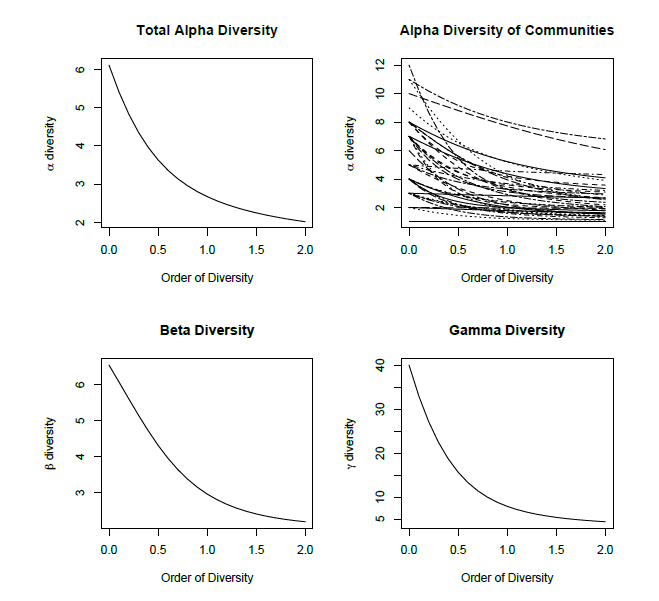
Three interesting values are q = 0, q = 1 and q = 2 corresponding to the most widely used entropy measures: the number of species, Shannon and Simpson. Let's start with q = 1. The first step is to compute the $\alpha$ diversity

> Alpha.dat.1=AlphaEntropy(q=1,MC=Meta.dat.st,Correction="ChaoShen")$Communities

To simplify the subsequent command writing, it is good practice to apply the attach function to the env data frame, in this way data frame columns become directly available in the current R session.

> attach(env)

To explore the relation between the $\alpha$ diversity and the three geological regions it is convenient to draw the box plot against the grouping factor:

> boxplot(Alpha.dat.1~Morphoregion,col=rainbow(3))

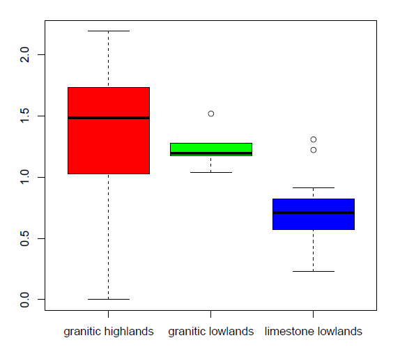
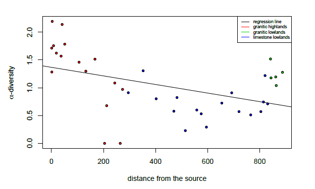
The plot suggests considerable difference between the limestone lowlands region and the other two. In a linear model this would imply at least a different intercept fro each region. Exploring the relation between $\alpha$ biodiversity and the environmental variables Distance and Altitude, the same suggestion is obtained:

> plot(Distance,Alpha.dat.1,pch=20,xlab="distance from the source",
+ ylab=expression(paste(alpha,"-diversity")))
> abline(lm(Alpha.dat.1~Distance))
> points(Distance,Alpha.dat.1,pch=20,col=c(2,3,4)[Morphoregion],cex=0.5)
> legend("topright",c("regression line",levels(Morphoregion)),lty=c(1),lwd=c(1,1,1,1),
+ col=c(1,2,3,4),cex=0.6)

> plot(Altitude,Alpha.dat.1,pch=20,xlab="Altitude",
+ ylab=expression(paste(alpha,"-diversity")))
> abline(lm(Alpha.dat.1~Altitude))
> points(Altitude,Alpha.dat.1,pch=20,col=c(2,3,4)[Morphoregion],cex=0.5)
> legend("bottomright",c("regression line",levels(Morphoregion)),
+ lty=c(1),lwd=c(1,1,1,1),col=c(1,2,3,4),cex=0.6)

Notice that the labels with greek letters are obtained using the function expression applied to the combination of the greek letter and the word diversity given by the function paste: expression(paste(alpha,"-diversity")). The lm function estimates linear models (simple regression), it returns objects of class lm such that:

> summary(lm(Alpha.dat.1~Distance))

Call:
lm(formula = Alpha.dat.1 ~ Distance)
Residuals:

Min	1Q	Median	3Q	Max
-1.20921	-0.25141	-0.00544	0.34443	0.82726

Coefficients:
Estimate Std. Error t value Pr(>|t|)
(Intercept) 1.3665728 0.1359560 10.052 5.41e-12 ***
Distance -0.0007714 0.0002549 -3.026 0.00455 **
---
Signif. codes: 0

The summarized output includes

the call to the lm function
basic statistics on model residuals (residuals are defined as fitted values - observed values)
the table of estimated coeficients, with standard errors and tests verifying if each coeficient is significantly different from zero
the measure of goodness of fit given by the R2 and its corrected version
the F test for the overall significance of the model

The quality of the fit is scarce, with a very small value of the R2. For the model with altitude:

> summary(lm(Alpha.dat.1~Altitude))

Call:
lm(formula = Alpha.dat.1 ~ Altitude)
Residuals:

Min	1Q	Median	3Q	Max
-1.0412	-0.2304	-0.0188	0.3617	0.7660

Coefficients:
Estimate Std. Error t value Pr(>|t|)
(Intercept) 0.7353361 0.0909699 8.083 1.32e-09 ***
Altitude 0.0008496 0.0001698 5.004 1.48e-05 ***
---
Signif. codes: 0 '***' 0.001 '**' 0.01 '*' 0.05 '.' 0.1 ' ' 1
Residual standard error: 0.4236 on 36 degrees of freedom
Multiple R-squared: 0.4102, Adjusted R-squared: 0.3938
F-statistic: 25.04 on 1 and 36 DF, p-value: 1.484e-05

To estimate a linear model with fixed effect ruled by the distance form the source and a random intercept ruled by the regions, it is necessary to call the package nlme and its function lme.

> require(nlme) > mod.1d=lme(Alpha.dat.1~Distance,random=~1|Morphoregion,method="ML") > mod.1a=lme(Alpha.dat.1~Altitude,random=~1|Morphoregion,method="ML")

the function lme accepts two estimation methods: ML and REML. In the following the ML method is going to be preferred. Model comparison is done using the Akaike Information criterion AIC which value can be retrieved from the lme output using the function with the same name or the summary function. The smallest the AIC the better the model. In the summary of a linear mixed model the same table of coeficients estimates as with the lm function is given, plus some additional features: (1) the model evaluation criteria AIC, BIC1 and log likelihood; (2) the portion of standard deviation represented by the ran- dom terms in the model and the residual standard deviation; (3) the correlation between the model coeficients; (4) some information about the groups:

> summary(mod.1d)

Linear mixed-effects model fit by maximum likelihood
Data: NULL

AIC	BIC	logLik
57.50108	64.05142	-24.75054

Random effects:
Formula: ~1 | Morphoregion
(Intercept) Residual
StdDev: 0.2550837 0.4357859
Fixed effects: Alpha.dat.1 ~ Distance
Value Std.Error DF t-value p-value
(Intercept) 1.5041056 0.2608184 34 5.766870 0.0000
Distance -0.0008709 0.0003963 34 -2.197679 0.0349
Correlation:
(Intr)
Distance -0.753
Standardized Within-Group Residuals:

Min	Q1	Med	Q3	Max
-2.86432169	-0.31961738	0.01304856	0.53776243	1.76284917

Number of Observations: 38
Number of Groups: 3

> summary(mod.1a)

Linear mixed-effects model fit by maximum likelihood
Data: NULL

AIC	BIC	logLik
46.59625	53.1466	-19.29813

Random effects:
Formula: ~1 | Morphoregion
(Intercept) Residual
StdDev: 0.2235278 0.3772537
Fixed effects: Alpha.dat.1 ~ Altitude
Value Std.Error DF t-value p-value
(Intercept) 0.7884804 0.16403300 34 4.806840 0e+00
Altitude 0.0009397 0.00021899 34 4.290888 1e-04
Correlation:
(Intr)
Altitude -0.404
Standardized Within-Group Residuals:

Min	Q1	Med	Q3	Max
-2.6545275	-0.4093024	0.1123792	0.5077570	2.0134121

Number of Observations: 38
Number of Groups: 3

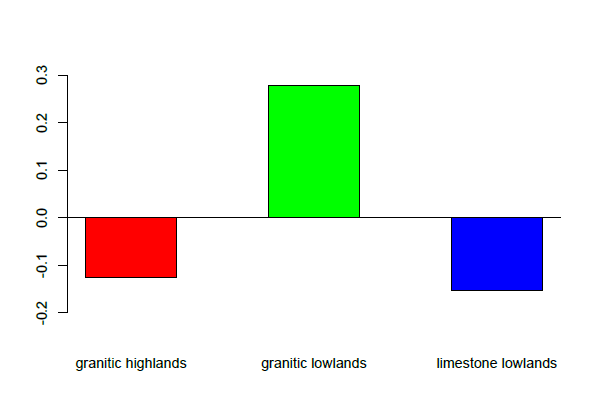
The model with Altitude has smaller AIC value. Plotting the three estimated intercepts shows that they are very similar for the groups granitic highlands and limestone lowlands, while granitic lowlands has fewer monitoring stations but a systematically larger $\alpha$ diversity value:

> barplot(t(mod.1a$coefficients$random$Morphoregion),beside=T,
+ col=rainbow(3),ylim=c(-0.25,0.3))
> abline(h=0)

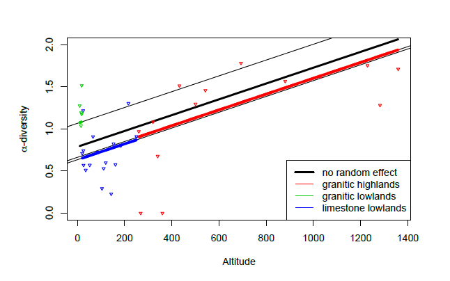
Plotting the model and the data together highlights a possible model improvement by considering a random intercept as well:

> F0=fitted(mod.1a,level=0)
> F1=fitted(mod.1a,level=1)
> I=order(Altitude)
> DD=sort(Altitude)
> plot(DD,F0[I],lwd=3,type="l",ylim=c(0,2),xlab="Altitude",
+ ylab=expression(paste(alpha,"-diversity")))
> aa=levels(Morphoregion)
> colo=c(2,3,4)
> for(i in 1:length(aa)){ + x1=Altitude[Morphoregion==aa[i]] + y1=F1[Morphoregion==aa[i]] + K=order(x1) + lines(sort(x1),y1[K],col=colo[i],lwd=4,lty=5) + abline(lm(y1[K]~sort(x1)),col=1,lwd=1) + lines(sort(x1),y1[K],col=colo[i],lwd=4) + + }
> points(Altitude,Alpha.dat.1,pch=25,col=c(2,3,4)[Morphoregion],cex=0.5)
> legend("bottomright",c("no random effect",aa),
+ lwd=c(3,1,1,1),col=c(1,2,3,4))

The model with random intercept and slope is estimated using the following syntax:

> mod.1as=lme(Alpha.dat.1~Altitude,random=~1+Altitude|Morphoregion,method="ML")
> summary(mod.1as)

Linear mixed-effects model fit by maximum likelihood Data: NULL

AIC	BIC	logLik
49.54251	59.36803	-18.77126

Random effects: Formula: ~1 + Altitude | Morphoregion Structure: General positive-definite, Log-Cholesky parametrization

	StdDev	Corr
(Intercept)	0.2569540925	(Intr)
Altitude	0.0002928191	-0.983
Residual	0.3744337217

Fixed effects: Alpha.dat.1 ~ Altitude

	Value	Std.Error	DF	t-value	p-value
(Intercept)	0.7888486	0.17856188	34	4.417788	0.0001
Altitude	0.0007965	0.00023974	34	3.322493	0.0021

Correlation:

	(Intr)
Altitude	-0.842

Standardized Within-Group Residuals:

Min	Q1	Med	Q3	Max
-2.6323065	-0.4035367	0.1089191	0.4684097	2.0412254

Number of Observations: 38 Number of Groups: 3

The AIC of this model is larger than the one with the random intercept alone. Plotting the model results it is clear that two out of three groups have overlapping regression lines and the granitic lowlands community provides only slight evidence of a different behavior (fewer stations with a very narrow altitude range). Also notice the very high correlation between the random intercepts and the random slope (-0.0983) meaning that this parametrization has some unnecessary redundancy.

Modelli misti con nlme

Lo scopo di questa unitá é quello di familiarizzare con la stima dei modelli ad effetti misti, in particolare l'uso della librerianlme. Gli esempi saranno eseguiti utilizzando i dataset del pacchetto ade4 usato nell'unitá precedente. Per primo si caricare la libreria e rendere il dataset disponibile per la sessione di lavoro corrente.

> require(ade4)
> data(macroloire)
> dat.1=macroloire$fau
> env=macroloire$envir

Questa volta la biodiversitá é misurata a livello di stazione di monitoraggio e l'intersse é quello di capire la variazione della diversitá ($\alpha$-diversity) come funzione dei fattori ambientali. Le stazioni di monitoraggio raggruppati in tre comunitá in corrispondenza delle regioni definiti in base alla geologia. il dataset env é il dataframe resituito per ogni stazione di monitoraggio:

il nome (variabile SamplingSite);
la distanza dalla fonte(km, variabile Distance);
l'altitudine (m, variabile Altitude);
la posizione delle dighe nei fiumi(variabile Dam):
1. prima della prima diga;
2. dopo la prima diga
3. Dopo la deconda digaam;
la posizione in uno delle tre regioni definiti in base alla geologia (variabile Morphoregion):
1. Altopiano granitico;
2. pianura calcare;
3. pianura granitica;
presenza di confluenti (variaile Confluence).

Per prima cosa si vuole misurare la biodiversiutá sulla scala spaziale della stazione di monitoraggio. Successivamente si definisce la meta-comunitá con le comunitá corrispondenti alle stazioni di monitoraggio:

> require(entropart)
> Meta.dat.st=MetaCommunity(dat.1,Weights=apply(dat.1,2,sum))

Per scegliere l'ordine di diversitá da usare, puó essere disegnare sul grafico i profili di diversitá:

> qq=seq(0,2,by=0.1)
> DivP.dat=DivProfile(qq,Meta.dat.st)

> plot(DivP.dat)

Tre valori interessanti sono q = 0, q = 1 e q = 2 che corrispondono ai valori di entropia piú usati: il numero delle specie, Shannon e Simpson. Si inizi con valutare q = 1. Pertanto si procede al calcolo della diversitá $\alpha$

> Alpha.dat.1=AlphaEntropy(q=1,MC=Meta.dat.st,Correction="ChaoShen")$Communities

Per semplificare la scrittura dei successivi comandi, é buona norma usare la funzione attach() al dataframe env, in questo modo le colonne del dataframe diventano direttamente disponibili nella sessione corrente di R.

> attach(env)

Per esaminare la relazione tra la diversitá $\alpha$ e le tre regioni geologiche é opportuno disegnare un box-plot rispetto ai fattori di raggruppamento:

> boxplot(Alpha.dat.1~Morphoregion,col=rainbow(3))

Il grafico suggerisce differenze consistenti fra i bassopiani calcarei e gli altri due. In un modello lineare questo avrebbe determinato almeno una intersezionene per ogni regione. Esaminando la relazione della biodiversitá $\alpha$ e le variabili ambientali Distance(Distanza) e Altitude(Altitudine), lo stesso suggerimento si ottiene:

Si noti che le etichette con le lettere greche sono ottenute usando la funzione expression applicata alla combinazione delle lettere greche e la paroloa "diversitá" data dalla funzione paste: expression(paste(alpha,"-diversity")). La funzione lm valuta i modelli lineari (regressione semplice), restituisce un oggetto della classe lm:

> summary(lm(Alpha.dat.1~Distance))

Call:
lm(formula = Alpha.dat.1 ~ Distance)
Residuals:

Min	1Q	Median	3Q	Max
-1.20921	-0.25141	-0.00544	0.34443	0.82726

Coefficients:
Estimate Std. Error t value Pr(>|t|)
(Intercept) 1.3665728 0.1359560 10.052 5.41e-12 ***
Distance -0.0007714 0.0002549 -3.026 0.00455 **
---
Signif. codes: 0

L'output riepilogativo include

la chiamata della funzione lm
statistiche base sui residui del modello (residui definiti come valori adattati- valori osservati)
la tabella dei coefficienti stimati, con errori standard e verifiche se ogni coefficiente e significativamente differente da zero
la misura della bontá di un adattamento dato da R² e la sua versione corretta
Il test F per il valore complessivo del modello

Se la qualitá dell'adattamento (fit) é scarsa, con un valore basso di R². Per il modello con altitudine:

> summary(lm(Alpha.dat.1~Altitude))

Call:
lm(formula = Alpha.dat.1 ~ Altitude)
Residuals:

Min	1Q	Median	3Q	Max
-1.0412	-0.2304	-0.0188	0.3617	0.7660

Per stimare un modello lineare con effetto fisso guidato dalla distanza della fonte ed intersezioni casuali guidate dalle regioni, é necessario richiamare il pacchetto nlme e la sua funzione lme.

> require(nlme) > mod.1d=lme(Alpha.dat.1~Distance,random=~1|Morphoregion,method="ML") > mod.1a=lme(Alpha.dat.1~Altitude,random=~1|Morphoregion,method="ML")

La funzione lme accetta due metodi di stima: ML e RML. Di seguito sará preferito il metodo ML. Il confronto fra modelli é effettuato utilizzando il criterio di informazione di Aikaike (AIC) il cui valore puó essere ricavato dall'output di lme utilizzando la funzione omonima o la funzione summary. Minore é l'AIC, tanto migliore é il modello. Nel riepilogo del modello lineare misto la stessa tabella dei coefficienti di stima é data come con la funzione lm, piú alcune funzionalitá aggiuntive: (1) i criteri di valutazione del modello AIC, BIC¹ e il log di verosomiglianza; (2) la porzione della deviazione standard rappresentata dai termini casuali nel modello e dalla deviazione standard dei residui; (3) la corelazione tra i coefficienti del modello; (4) alcune informazioni sui gruppi:

> summary(mod.1d)

Linear mixed-effects model fit by maximum likelihood
Data: NULL

AIC	BIC	logLik
57.50108	64.05142	-24.75054

Min	Q1	Med	Q3	Max
-2.86432169	-0.31961738	0.01304856	0.53776243	1.76284917

Number of Observations: 38
Number of Groups: 3

> summary(mod.1a)

Linear mixed-effects model fit by maximum likelihood
Data: NULL

AIC	BIC	logLik
46.59625	53.1466	-19.29813

Min	Q1	Med	Q3	Max
-2.6545275	-0.4093024	0.1123792	0.5077570	2.0134121

Number of Observations: 38
Number of Groups: 3

Il modello con l'altitudine ha un valore inferiore di AIC. Disegnando i le tre intersezioni stimate si nota che sono molto simili per i gruppi dell'altopiano granitico e quello del bassopiano calcareo, mentre il bassopino granitico ha meno stazioni di monitoraggio ma sistematicamente un valore di diversitá $\alpha$ ampio:

> barplot(t(mod.1a$coefficients$random$Morphoregion),beside=T,
+ col=rainbow(3),ylim=c(-0.25,0.3))
> abline(h=0)

Disegnando il modello insieme ai dati, evidenzia una possibile miglioria del modello utilizzando una intersezione casuale:

Il modello con l'intersezione e inclinazione casuale é stimata utilizzando la seguente sintassi:

> mod.1as=lme(Alpha.dat.1~Altitude,random=~1+Altitude|Morphoregion,method="ML")
> summary(mod.1as)

Linear mixed-effects model fit by maximum likelihood Data: NULL

AIC	BIC	logLik
49.54251	59.36803	-18.77126

Random effects: Formula: ~1 + Altitude | Morphoregion Structure: General positive-definite, Log-Cholesky parametrization

	StdDev	Corr
(Intercept)	0.2569540925	(Intr)
Altitude	0.0002928191	-0.983
Residual	0.3744337217

Fixed effects: Alpha.dat.1 ~ Altitude

	Value	Std.Error	DF	t-value	p-value
(Intercept)	0.7888486	0.17856188	34	4.417788	0.0001
Altitude	0.0007965	0.00023974	34	3.322493	0.0021

Correlation:

	(Intr)
Altitude	-0.842

Standardized Within-Group Residuals:

Min	Q1	Med	Q3	Max
-2.6323065	-0.4035367	0.1089191	0.4684097	2.0412254

Number of Observations: 38 Number of Groups: 3

L'AIC di questo modello é maggiore di quello con la sola intersezione casuale. Disegnando i risultati del modello é evidente che due dei tre gruppo hanno linee di regressione sovrapposte e che la comunitá del bassopiano granitico fornisce solo una piccola prova di un comportamento differente (meno stazioni con altitudini vicine). Si noti anche la alta correlazione fra le intersezioni casuali e le inclinazioni casuali (-0.0983) significato che questa parametrizazione ha della rindondanza non necessaria.