Data Management and Biodiversity partitioning using the R package entropart - Gestione dati e partizione della biodiversità con il package entropart di R
The entropart package
To obtain information on the entire dataset it is useful to define a Meta-community as available in the entropart package.
> library(entropart)
Meta-communities can be built giving equal or different weights to the communities. Weights can be chosen arbitrarily but usually they are proportional to the number of individuals found in each community. Equally weighted communities are obtained as:
> Meta.dat2=MetaCommunity(dat.2,Weights=c(1,1,1))
For objects of class MetaCommunity the summary and plot functions have specific methods:
> summary(Meta.dat2)
Meta-community (class 'MetaCommunity') made of 4785 individuals in 3 communities and 40 species.
Its sample coverage is 0.99914310220727
Community weights are:
| granitic highlands | granitic lowlands | limestone lowlands |
| 0.3333333 | 0.3333333 | 0.3333333 |
Community sample numbers of individuals are:
| granitic highlands | granitic lowlands | limestone lowlands |
| 1595 | 747 | 2324 |
Community sample coverages are:
| granitic highlands | granitic lowlands | limestone lowlands |
| 0.9981231 | 0.9973226 | 0.9987102 |
> plot(Meta.dat2,col=rainbow(40))
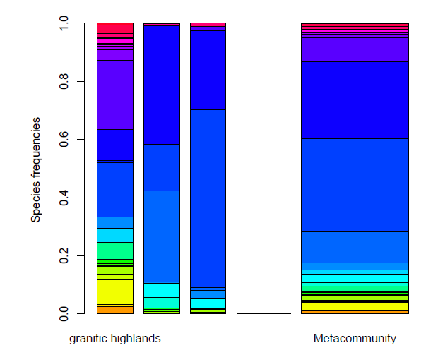
Notice the difference when the communities are weighted. Here we choose weights proportional to the number of individuals in each community:
> ww=c(1595,747,2324 )/(1595+747 +2324 ) > Meta.dat2a=MetaCommunity(dat.2,Weights=ww) > summary(Meta.dat2)
Meta-community (class 'MetaCommunity') made of 4666 individuals in 3 communities and 40 species.
Its sample coverage is 0.99914310220727
Community weights are:
| granitic highlands | granitic lowlands | limestone lowlands |
| 0.34183453 | 0.1600943 | 0.4980712 |
Community sample numbers of individuals are:
| granitic highlands | granitic lowlands | limestone lowlands |
| 1595 | 747 | 2324 |
Community sample coverages are:
| granitic highlands | granitic lowlands | limestone lowlands |
| 0.9981231 | 0.9973226 | 0.9987102 |
> plot(Meta.dat2,col=rainbow(40))
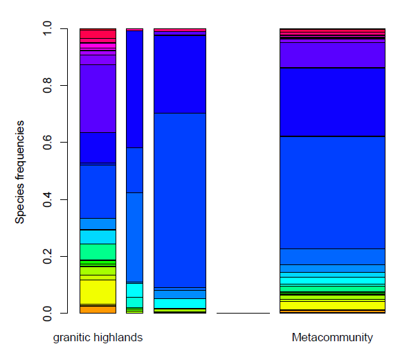
When meta-communities are built with this faunistic table a warning message is issued, as there is one species that is largely more abundant then the others in the third community (limestone lowlands), as can be seen by computing the community relative abundances:
> rela=dat.2[,3]/sum(dat.2[,3])
This unbalance creates a problem in the computation of bias corrections. Another interesting quantity that can be computed from the meta commu- nity object is the sample coverage, that is almost 1 in the current dataset for the three communities and for the metacommunity:
> Coverage(Ns=Meta.dat2$Ns)
[1] 0.9991627
In the macroloire list the names of the species are in the data frame element macroloire$labels. To associate species names to the above vector's elements consider that macroloire$labels is a data frame object and has to be addressed using the appropriate syntax:
> names(rela)=as.character(macroloire$labels[,1])
> rela
| Potamophilus acuminatus | Stenelmis canaliculata | Macronychus quadrituberculatus | Dupophilus brevis |
| 0.0008605852 | 0.0030120482 | 0.0017211704 | 0.0000000000 |
| Elmis aenea | Elmis maugetii | Elmis rioloides | Esolus angustatus |
| 0.0000000000 | 0.0000000000 | 0.0000000000 | 0.0000000000 |
| Esolus parallelepipedus | Esolus pygmaeus | Limnius perrisi | Limnius volckmari |
| 0.0004302926 | 0.0090361446 | 0.0000000000 | 0.0008605852 |
| Limnius opacus | Oulimnius troglodytes | Oulimnius tuberculatus | Platambus maculatus |
| 0.0004302926 | 0.0017211704 | 0.0000000000 | 0.0000000000 |
| Oreodytes sanmarkii | Oligoplectrum maculatum | Micrasema longulum | Ecnomus deceptor |
| 0.0000000000 | 0.0000000000 | 0.0000000000 | 0.0008605852 |
| Ecnomus tenellus | Glossosoma conformis | Agapetus delicatulus | Cheumatopsyche lepida |
| 0.0339931153 | 0.0000000000 | 0.0000000000 | 0.0275387263 |
| Hydropsyche bulgaromanorum | Hydropsyche contubernalis | Hydropsyche dinarica | Hydropsyche exocellata |
| 0.0107573150 | 0.6114457831 | 0.0000000000 | 0.2723752151 |
| Hydropsyche ornatula | Hydropsyche pellucidula | Hydropsyche siltalai | Allogamus auricollis |
| 0.0017211704 | 0.0116179002 | 0.0000000000 | 0.0000000000 |
| Chimarra marginata | Philopotamus montanus | Polycentropus flavomaculatus | Plectrocnemia geniculata |
| 0.0000000000 | 0.0000000000 | 0.0000000000 | 0.0000000000 |
| Neureclipsis bimaculata | Psychomyia pusilla | Rhyacophila praemorsa | Thremma gallicum |
| 0.0004302926 | 0.0111876076 | 0.0000000000 | 0.0000000000 |
The Hydropsyche contubernalis has a relative abundance of 0.611. Now consider a new faunistic table, namely the dataset jv73 of the package ade4:
This data set gives physical and physico-chemical variables, fish species, spatial coordinates about 92 sites. It is a list of 6 components:
- morpho is a data frame with 92 sites and 6 physical variables.
- phychi is a data frame with 92 sites and 12 physico-chemical variables.
- poi is a data frame with 92 sites and 19 fish species.
- xy is a data frame with 92 sites and 2 spatial coordinates.
- contour is a data frame for mapping.
- fac.riv is a factor distributing the 92 sites on 12 rivers.
As before the interest is in communities with spatial scale larger than the monitoring station. Communities are defined by each of 12 rivers, then it is necessary to create a new faunistic table with abundances (number of individuals here) aggregated by river. As in the previous example, it is convenient to extract the faunistic table from the list and then build the cycle:
> data(jv73)
> app=t(jv73$poi)
> jv73.fau=data.frame(matrix(0,nrow(app),ncol=12))
> for(i in 1:nrow(app)){
+ jv73.fau[i,]=tapply(t(app[i,]),jv73$fac.riv,sum)
+ }
> colnames(jv73.fau)=levels(jv73$fac.riv)
> row.names(jv73.fau)=row.names(app)
In the object jv73.fau the 12 communities are ready to be analyzed.
> apply(jv73.fau,2,sum)
| Allaine | Audeux | Clauge | Cuisance | Cusancin | Dessoubre |
| 52 | 37 | 124 | 72 | 37 | 53 |
| Doubs | Doulonnes | Drugeon | Furieuse | Lison | Loue |
| 302 | 35 | 96 | 66 | 80 | 409 |
Notice that very different abundances are observed in the 12 communities:
> ww.jv=apply(jv73.fau,2,sum)/(sum(apply(jv73.fau,2,sum) ))
This suggests the construction of a weighted meta-community, obtained with following syntax:
> Meta.jv=MetaCommunity(jv73.fau,Weights=ww.jv)
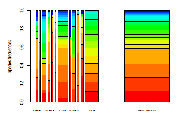
To plot the meta-community giving one color to each species it is convenient to build a color palette. The function colorRampPalette allows to build the desired graduated color scale:
> plot(Meta.jv,col=colorRampPalette(c("red","yellow","green","cyan","blue"))(19), + cex.names=0.5)
To get familiar with the entropart package it is useful to experiment with some of its functions. To compute Tsallis entropies there is the function with the same name
> Tsallis(Ps=Meta.jv$Ps,q=1)
[1] 2.551949
Same as:
> Shannon(Ps=Meta.jv$Ps)
[1] 2.551949
To apply the bias correction write:
> bcTsallis(Ns=Meta.jv$Ns,q=1)
[1] 2.555498
> bcShannon(Ns=Meta.jv$Ns)
[1] 2.555498
Notice that no differences are found when the coverage is almost 1, i.e no singletons are found in the faunistic table
> Coverage(Ns=Meta.jv$Ns)
[1] 1
To compute the Hill numbers corresponding to the Simpson index (Tsallis entropy with q = 2 or also the Gini's index introduced in 1920's to study income distributions) write:
> expq(Tsallis(Ps=Meta.jv$Ps,q=2),q=2)
[1] 9.906675
that is the same as
> Diversity(Ps=Meta.jv$Ps,q=2)
[1] 9.906675
To apply the bias correction to the diversity measure:
> bcDiversity(Ns=Meta.jv$Ns,q=2)
[1] 9.979207
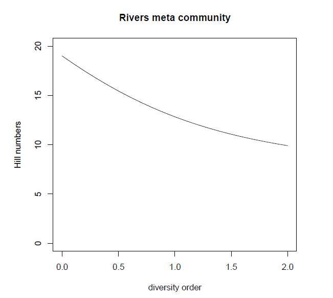
The corrected diversities can be interpreted extending the idea of effective number of species, or Hill numbers. They can be examined with different types of plots.
The schematic procedure is:
- prepare a vector with the diversities order
- compute the diversity profile using DivProfile
- extract the gamma diversity from the diversity profile object
- plot the gamma diversity vs the diversities order
> qq=seq(0,2,by=0.1)
> dd=DivProfile(qq,Meta.jv)
> names(dd)
| [1] | "MetaCommunity" | "Order" | "Biased" | "Correction" | "Normalized" |
| [6] | "TotalAlphaDiversity" | "TotalBetaDiversity" | "GammaDiversity" | "TotalAlphaEntropy" | "TotalBetaEntropy" |
| [11] | "GammaEntropy" |
> plotHn=dd$GammaDiversity
> plot(qq,plotHn,type="l",ylim=c(0,20),xlab="diversity order",
+ylab="Hill numbers",main="Rivers meta community")
Il pacchetto entropart
Per ottenere informazioni sull'intero data set é utile definire una meta-comunitá come "disponibile" nel pacchetto entropart.
> library(entropart)
Meta-comunitá possono essere create dando pesi uguali o differenti alle comunitá. I pesi possono essere scelti arbitrariamente, ma in genere sono proporzionali al numero di esemplari popolanti la singola comunitá. Comunitá con pesi uguali sono ottenuti come:
> Meta.dat2=MetaCommunity(dat.2,Weights=c(1,1,1))
Per oggetti della classe MetaComunity le funzioni summary e plot hanno metodi specifici:
> summary(Meta.dat2)
Meta-community (class 'MetaCommunity') made of 4785 individuals in 3 communities and 40 species.
Its sample coverage is 0.99914310220727
Community weights are:
| granitic highlands | granitic lowlands | limestone lowlands |
| 0.3333333 | 0.3333333 | 0.3333333 |
Community sample numbers of individuals are:
| granitic highlands | granitic lowlands | limestone lowlands |
| 1595 | 747 | 2324 |
Community sample coverages are:
| granitic highlands | granitic lowlands | limestone lowlands |
| 0.9981231 | 0.9973226 | 0.9987102 |
> plot(Meta.dat2,col=rainbow(40))
Notice the difference when the communities are weighted. Here we choose weights proportional to the number of individuals in each community:
> ww=c(1595,747,2324 )/(1595+747 +2324 ) > Meta.dat2a=MetaCommunity(dat.2,Weights=ww) > summary(Meta.dat2)
Meta-community (class 'MetaCommunity') made of 4666 individuals in 3 communities and 40 species.
Its sample coverage is 0.99914310220727
Community weights are:
| granitic highlands | granitic lowlands | limestone lowlands |
| 0.34183453 | 0.1600943 | 0.4980712 |
Community sample numbers of individuals are:
| granitic highlands | granitic lowlands | limestone lowlands |
| 1595 | 747 | 2324 |
Community sample coverages are:
| granitic highlands | granitic lowlands | limestone lowlands |
| 0.9981231 | 0.9973226 | 0.9987102 |
> plot(Meta.dat2,col=rainbow(40))
Quando sono create meta-comunitá con questa tabella faunistica, viene lanciato un messaggio di avvertimento (warning), siccome una specie é molto piú abbondante che le altre nella terza comunitá (bassopiano calcareo), come si puó vedere calcolando le abbondanze relative della comunitá:
> rela=dat.2[,3]/sum(dat.2[,3])
Questo sbilanciamento crea problemi nel calcolo delle correzioni degli errori (bias). Un altro interessante valore che puó essere calcolato dall'oggetto meta-comunitá é la copertura campionaria, che é pressoché 1 nel dataset corrente per le tre comunitá e per la metacomunitá:
> Coverage(Ns=Meta.dat2$Ns)
[1] 0.9991627
Nella lista macroloire i nome delle specie sono indicate nell'elemento del dataframe macroloire$labels. Per associare i nomi delle specie agli elementi del vettore precedente si consideri che macroloire$labels é un oggetto del dataframe e deve essere indirizzato con un adeguata sintassi:
> names(rela)=as.character(macroloire$labels[,1])
> rela
| Potamophilus acuminatus | Stenelmis canaliculata | Macronychus quadrituberculatus | Dupophilus brevis |
| 0.0008605852 | 0.0030120482 | 0.0017211704 | 0.0000000000 |
| Elmis aenea | Elmis maugetii | Elmis rioloides | Esolus angustatus |
| 0.0000000000 | 0.0000000000 | 0.0000000000 | 0.0000000000 |
| Esolus parallelepipedus | Esolus pygmaeus | Limnius perrisi | Limnius volckmari |
| 0.0004302926 | 0.0090361446 | 0.0000000000 | 0.0008605852 |
| Limnius opacus | Oulimnius troglodytes | Oulimnius tuberculatus | Platambus maculatus |
| 0.0004302926 | 0.0017211704 | 0.0000000000 | 0.0000000000 |
| Oreodytes sanmarkii | Oligoplectrum maculatum | Micrasema longulum | Ecnomus deceptor |
| 0.0000000000 | 0.0000000000 | 0.0000000000 | 0.0008605852 |
| Ecnomus tenellus | Glossosoma conformis | Agapetus delicatulus | Cheumatopsyche lepida |
| 0.0339931153 | 0.0000000000 | 0.0000000000 | 0.0275387263 |
| Hydropsyche bulgaromanorum | Hydropsyche contubernalis | Hydropsyche dinarica | Hydropsyche exocellata |
| 0.0107573150 | 0.6114457831 | 0.0000000000 | 0.2723752151 |
| Hydropsyche ornatula | Hydropsyche pellucidula | Hydropsyche siltalai | Allogamus auricollis |
| 0.0017211704 | 0.0116179002 | 0.0000000000 | 0.0000000000 |
| Chimarra marginata | Philopotamus montanus | Polycentropus flavomaculatus | Plectrocnemia geniculata |
| 0.0000000000 | 0.0000000000 | 0.0000000000 | 0.0000000000 |
| Neureclipsis bimaculata | Psychomyia pusilla | Rhyacophila praemorsa | Thremma gallicum |
| 0.0004302926 | 0.0111876076 | 0.0000000000 | 0.0000000000 |
La Hydropsyche contubernalis ha una abondanza relativa di 0.611. Si consideri una nuova tabella faunistica, ossia il dataset jv73 del pacchetto ade4:
Questo dataset fornisce viariabili fisiche e fisico-chimiche, specie di pesci, coordianate spaziale di circa 92 siti. É una lista di 6 componenti:
- morpho é un dataframe con 92 siti e 6 variabili fisiche.
- phychi é un dataframe con 92 siti e 12 variabili fisico-chimiche.
- poi é un dataframe con 92 siti e 19 specie di pesci.
- xy é un dataframe con 92 siti e 2 coordinate spaziali.
- contour é un dataframe per la mappatura.
- fac.riv é un fattore che distribuisce i 92 siti su 12 fiumi.
Siccome, come prima, l'interesse é per le comunitá con una scala spaziale maggiore di una stazione di monitoraggio. Comunitá sono definite da ogniuno dei 12 fiumi, quindi é necessario creare una nuova tabella faunistica con le abbondanze (numero di esemplari) aggragati dal fiume. Come nell'esempio precedente, é opportuno estrarre la tabella faunistica dalla lista e poi creare il ciclo:
> data(jv73)
> app=t(jv73$poi)
> jv73.fau=data.frame(matrix(0,nrow(app),ncol=12))
> for(i in 1:nrow(app)){
+ jv73.fau[i,]=tapply(t(app[i,]),jv73$fac.riv,sum)
+ }
> colnames(jv73.fau)=levels(jv73$fac.riv)
> row.names(jv73.fau)=row.names(app)
Nell'oggetto jv73.fau le 12 comunitá sono pronte ad essere analizzate.
> apply(jv73.fau,2,sum)
| Allaine | Audeux | Clauge | Cuisance | Cusancin | Dessoubre |
| 52 | 37 | 124 | 72 | 37 | 53 |
| Doubs | Doulonnes | Drugeon | Furieuse | Lison | Loue |
| 302 | 35 | 96 | 66 | 80 | 409 |
Si osservano abbondanze molto differenti nelle 12 comunitá:
> ww.jv=apply(jv73.fau,2,sum)/(sum(apply(jv73.fau,2,sum) ))
Questo suggerisce la costruzione di una meta-comunitá ponderata, ottenuta con la seguente sintassi:
> Meta.jv=MetaCommunity(jv73.fau,Weights=ww.jv)
Per disegnare una meta-comunitá specificando un colore per ogni specie é opportuno creare una palette di colori. La funzione colorRampPalette consente di realizzare la scala graduata di colori desiderata:
> plot(Meta.jv,col=colorRampPalette(c("red","yellow","green","cyan","blue"))(19), + cex.names=0.5)
Per familiarizzare con il pacchetto entropart é utile sperimentare con alcune delle sue funzioni. Per calcolare le entropie di Tsallis esiste una funzione che ha lo stesso nome:
> Tsallis(Ps=Meta.jv$Ps,q=1)
[1] 2.551949
Come anche:
> Shannon(Ps=Meta.jv$Ps)
[1] 2.551949
Per applicare la correzione del bias si scriva:
> bcTsallis(Ns=Meta.jv$Ns,q=1)
[1] 2.555498
> bcShannon(Ns=Meta.jv$Ns)
[1] 2.555498
Si noti che non ci sono differenze se la copertura é ciraca 1, ossia non vi sono esemplari singoli nella tabella faunistica:
> Coverage(Ns=Meta.jv$Ns)
[1] 1
Per calcolare i numeri di Hill corrispondenti all'indice di Simpson (entropia di Tsallis con q=2 oppure l'indice di Gini introdotto negli anni '20 per studiare la distribuzione dei reditti) si scriva:
> expq(Tsallis(Ps=Meta.jv$Ps,q=2),q=2)
[1] 9.906675
che é lo stessi a
> Diversity(Ps=Meta.jv$Ps,q=2)
[1] 9.906675
Per eseguire la correzione del bias al valore della diversitá:
> bcDiversity(Ns=Meta.jv$Ns,q=2)
[1] 9.979207
Le diversitá corrette posssono essere interpretate esetendendo il concetto di numero di specie effettive, o numeri di Hill: Possono essere esaminate con diversi tipi di grafici.
Lo schema delle procedure é:
- preparare un vettore con l'ordine delle diversitá
- calcolare il profilo della diversitá usando DivProfile
- estrarre la diversitá gamma dall'oggetto profilo di divesitá(diversity profile object)
- disegnare la difersitá gamma relazionata all'ordine (grado) di diversitá
> qq=seq(0,2,by=0.1)
> dd=DivProfile(qq,Meta.jv)
> names(dd)
| [1] | "MetaCommunity" | "Order" | "Biased" | "Correction" | "Normalized" |
| [6] | "TotalAlphaDiversity" | "TotalBetaDiversity" | "GammaDiversity" | "TotalAlphaEntropy" | "TotalBetaEntropy" |
| [11] | "GammaEntropy" |
> plotHn=dd$GammaDiversity
> plot(qq,plotHn,type="l",ylim=c(0,20),xlab="diversity order",
+ylab="Hill numbers",main="Rivers meta community")