Data Management and Biodiversity partitioning using the R package entropart - Gestione dati e partizione della biodiversità con il package entropart di R
Data Management
In the session Introduction to R we already saw how to read a text data file into R. We are now going to learn how to perform simple data manipulations in R. First of all we load into the workspace a dataset available package ade4, devoted to ecological analysis. By typing
> library(ade4)
> data(macroloire)
A total of 38 sites were surveyed along 800 km of the Loire River yielding 40 species of Trichoptera and Coleoptera sampled from riffle habitats. The river was divided into three regions according to ge- ology: granitic highlands (Region n.1), limestone lowlands (Region n.2) and granitic lowlands (Region n.3). This data set has been col- lected for analyzing changes in macroinvertebrate assemblages along the course of a large river. Four criteria are given here: variation in 1) species composition and relative abundance, 2) taxonomic composition, 3) Body Sizes, 4) Feeding habits.
Data are organized as elements of the macroloire list. In the faunistic table macroloire$fau , sites are on the columns and species on the rows. In the following examples interest is focused on communities defined by the grouping factor macroloire$envir$Morphoregion. Now in order to construct a faunistic table for the three regions, it is necessary to rearrange data so that abundances originally referred to monitoring stations are aggregated into the three commu- nities. First, in order to simplify the commands writing, extract the faunistic table and Morphoregion factor from the macroloire list:
> dat.1=macroloire$fau
> reg=macroloire$envir$Morphoregion
We want to sum abundances of each species recorded at sites, according to the region they belong to. For the first species in the macroloire faunistic table, i.e. the first row ofdat.1:
> tapply(t(dat.1[1,]),reg,sum)
| granitic highlands | granitic lowlands | limestone lowlands |
| 0 | 0 | 2 |
The function tapply allows to apply a function (in this case sum) to a vector according to a grouping factor [1]. Now we need to apply the same set of operations to each species, i.e. to each row of the faunistic table dat.1 Instead of manually doing this, it is easier to use a cycle. Cycles are useful whenever we need to replicate the same operation until a given condition is verified. The simplest and maybe most common situation is when we know exactly how many times an operation or a sequence of operations must be computed. The general structure of a cycle is for (k in 1:x){...}, where k is an index that will be incremented from 1 to x and the commands between curly brackets will be repeated x times.
We first create a new object with the same number of rows as dat.1 and 3 columns as communities in reg are 3. This object will become the new faunistic table.
> dat.2=matrix(0,nrow(dat.1),3)
The cycle implementing the construction of the faunistic table is:
> for(i in 1:nrow(dat.1)){
+ dat.2[i,]=tapply(t(dat.1[i,]),reg,sum)
+ }
> row.names(dat.2)=row.names(dat.1)
> colnames(dat.2)=levels(reg)
> dat.2=as.data.frame(dat.2)
The last three commands assign the species names to the rows of the new faunistic table, the names of the regions to its columns and transforms it into a data frame. As a first check we can verify it there are rare species in the dataset. This can be done by computing the total counts of the species (rows) in the dataset dat.2
> apply(dat.2,1,sum)
| E1 | E2 | E3 | E4 | E5 | E6 | E7 | E8 | E9 | E10 | E11 | E12 | E13 | |
| 2 | 7 | 4 | 1 | 40 | 4 | 8 | 134 | 29 | 75 | 2 | 8 | 13 | |
| E14 | E15 | E16 | E17 | E18 | E19 | E20 | E21 | E22 | E23 | E24 | E25 | E26 | |
| 24 | 4 | 1 | 1 | 90 | 2 | 29 | 115 | 77 | 1 | 130 | 259 | 1839 | |
| E27 | E28 | E29 | E30 | E31 | E32 | E33 | E34 | E35 | E36 | E37 | E38 | E39 | E40 |
| 10 | 1110 | 4 | 406 | 57 | 22 | 5 | 10 | 27 | 2 | 8 | 49 | 46 | 11 |
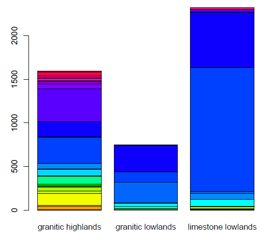
Several species are found only once or twice. Using the barplot function it is possible to visualize the distributions of the species in the three regions. The function requires an object of mode matrix as input that can be obtained calling the as.matrix() function in the the barplot command:
> barplot(as.matrix(dat.2),col=rainbow(40))
Gestione dei dati
Nella sezione "Introduzione a R" si é visto come importare un file dati di testo nell'ambiente di R. Ora si vedrÁ come effettuare delle semplici manipolazioni di dati in R. Per primo si carica nello spazio di lavoro un dataset disponibile nel package ade4, dedicato alle analisi ecologiche. Digitando
> library(ade4)
> data(macroloire)
Un totale di 38 siti sono stati censiti lungo 800 km del fiume della Loira, individuando 40 specie di Trichoptera e Coleoptera campionati dall'habitat che scorre. Il fiume é stato diviso in 3 regione in base alla sua geologia: gli altipiani granitici (Regione n.1), pianura calcarea (Regione n.2) e la pianura granitica (Regione n.3). Questo dataset é stato raccolto per analizzare cambiamenti dell'assembramento dei macroinvertebrati lungo il corso di un grande fiume. Sono dati 4 criteri: variazioni di 1) composizione delle specie e relativa abbondanza, 2) composizione tassonomica, 3) dimensioni corporali, 4) abitudini alimentari.
Nella lista macroloire i dati sono organizzati come elementi. Nella tabella faunistica macroloire$fau , i siti sono nelle colonne e le specie nelle righe. L'interesse del seguente esempio é focalizzato sulle comunitá definite da un fattore di raggruppamento macroloire$envir$Morphoregion. Per costruire una tabella faunistica per le tre regioni, é necessatrio riorganizzare i dati in modo che le abbondanze riferite alle stazioni di monitoraggio sono aggregate nelle tre comunitá. In modo da semplificare la digitazione dei comandi, si estraggono la tabella faunistica e il fattore Morphoregion dalla lista macroloire:
> dat.1=macroloire$fau
> reg=macroloire$envir$Morphoregion
Se si vogliono sommare le abbondanze di ogni specie registrate ai siti, tenendo conto della regione di appartenenza. Per la prima specie della tabella faunistica di macroloire, ossia il primo rigo di dat.1:
> tapply(t(dat.1[1,]),reg,sum)
| granitic highlands | granitic lowlands | limestone lowlands |
| 0 | 0 | 2 |
La funzione tapply permette di applicare un funzione (in questo caso sum) ad un vettore in base ad un fattore di raggruppamento [1]. Ora si applica lo stesso insieme di operazione ad orgni specie, ossia per ogni rigo della tabella faunistica dat.1. Invece di operare manualmente, é piú semplice utilizzare un ciclo. I cicli sono utili ogni qual volta si deve eseguire la stessa operazione finchè una determinata condizione non si verfichi. La piú semplice e piú comune situazione é quando si conosce il numero di volte che una operatzione o una sequenza di operazioni deve essere eseguita. La struttura generale di un ciclo é for (k in 1:x){...}, dove k é un indice che viene incrementato da 1 a x e i comandi fra parentesi graffe vengono ripetute x volte.
Per primo si crea un nuovo oggetto con lo stesso numero di rghi di dat.1 e 3 colonne siccome le comunitá in reg sono 3. Questo oggetto diventerá la nuova tabella faunistica.
> dat.2=matrix(0,nrow(dat.1),3)
Il ciclo che implementa la costruzione della tabella faunistica é:
> for(i in 1:nrow(dat.1)){
+ dat.2[i,]=tapply(t(dat.1[i,]),reg,sum)
+ }
> row.names(dat.2)=row.names(dat.1)
> colnames(dat.2)=levels(reg)
> dat.2=as.data.frame(dat.2)
Gli ultimi tre comandi assegnano i nomi delle specie alle righe della nuova tabella faunistica, i nome delle regioni alle sue colonne, trasformandola così in un data frame. Come primo controllo si puó verificare che vi sono specie rare presenti nel dataset. Ció si puó fare contando il numero di specie (righe) nel dataset dat.2
> apply(dat.2,1,sum)
| E1 | E2 | E3 | E4 | E5 | E6 | E7 | E8 | E9 | E10 | E11 | E12 | E13 | |
| 2 | 7 | 4 | 1 | 40 | 4 | 8 | 134 | 29 | 75 | 2 | 8 | 13 | |
| E14 | E15 | E16 | E17 | E18 | E19 | E20 | E21 | E22 | E23 | E24 | E25 | E26 | |
| 24 | 4 | 1 | 1 | 90 | 2 | 29 | 115 | 77 | 1 | 130 | 259 | 1839 | |
| E27 | E28 | E29 | E30 | E31 | E32 | E33 | E34 | E35 | E36 | E37 | E38 | E39 | E40 |
| 10 | 1110 | 4 | 406 | 57 | 22 | 5 | 10 | 27 | 2 | 8 | 49 | 46 | 11 |
Diverse specie sono state trovate solo una o due volte. Utilizzando la funzione barplot é possibile visualizzare la distribuzione delle specie nelle tre regioni. La funzione richiede un oggetto di modo matrix (matrixe) come dato di input e puó essere ottenuto invocando la funzione as.matrix() nel comando barplot:
> barplot(as.matrix(dat.2),col=rainbow(40))