Finite Markov Chains - Part I
Let Xt be a random variable describing the observation of some phenomenon at discrete times t = 1, 2, … . In the ecological framework, Xt could describe monthly abundance, yearly presence/absence, and so on. We further assume that Xt can only assume a finite set, x1, x2, …, xN, of values. For presence/absence data, N = 2, x1 = 0 (absence) and x2 = 1 (presence). By introducing a few thresholds, monthly abundances could be categorized in x1 = 0 (absence), x2 = 1 (low abundance), x3 = 2 (medium abundance) and x4 = 3 (high abundance), for instance.
The random process (Xt : t = 1,2, … ) is a discrete-time, finite-space, first order Markov Chain if at any time t, the future observation, Xt+1, depends on the past by the current observation, Xt , only [1].
In terms of conditional probability this can be fully stated as:
(2.1) P(Xt+1 = xi | X1 = xk,1 , … , Xt = xk,t) = P(Xt+1 = xi | Xt = xk,t)
(2.1) \(P(X_{t+1} = x_{i}| X_{1} = x_{k,1}, ..., X_{t} = x_{k,t})=P(X_{t+1} = x_{i}|X_{t} = x_{k,t})\)
for any time t, any value xi and any sequence of past observations (xk,1 , … , xk,t).
The conditional probability P(Xt+1 = xi | Xt = xk) will be also called transition (probability) from xk to xi at time t. Each xi is called a state and the set {<i> x</i><sub>1</sub>, <i>x</i><sub>2</sub>, <i>… </i>, <i>x<sub>N </sub></i>} of all the possible values of Xt is called state-space. We will write (Xt)t≥1, a notation usually applied to continuous-time processes, for the discrete-time process as continuous-time processes will not be considered in this course.
|
Example 2.1. Let (Xt)t≥1 the presence/absence process. Let (X1, X2, X3) = (1, 0, 1). Then P(X4 = 1 | X1 = 1 , X2 = 0, X3 = 1) = P(X4 = 1 | X3 = 1). |
As a direct consequence of (2.1), at any time t the conditional distribution of Xt+1 given the past (X1 , … , Xt) is fully defined by a matrix, the probability transition matrix (or simply transition matrix) Pt stating all the possible transitions pij from Xt = xi to Xt+1 = xk for i = 1, …, N and k = 1, … , N.
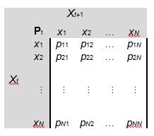
By definition, the matrix Pt is stochastic, that is the elements of any row sum to 1. Indeed pk1+ … + pkN is the sum of all the transitions that could occur at time t from xk to any state, including xk itself.
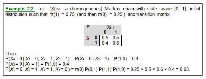
In general, the transitions pij depend on t. That is, P(X4 = 0 | X3 = 1) and P(X2 = 0 | X1 = 1) can differ each other, as the transition from 1 to 0 occur at different times. If Pt does not depend on time (Pt = P for all t ≥ 1) the Markov chain is called homogeneous. In other words, for a homogeneousMarkov chain, the probability of the future state of the chain only depends on the starting point. Hereafter we will only consider homogeneous Markov chain, and the term homogeneous will be omitted.
By applying the Bayes rule [2] and iterating (2.1), we can write
(2.2) P(X1 = xk,1 , … , Xt = xk,t , Xt+1 = xi ) =
P(Xt+1 = xi | Xt = xk,t) P(Xt = xk,t | Xt-1 = xk,t-1 ) … P(X2 = xk,2| X1 = xk,1) P(X1 = xk,1)
(2.2) \(P(X_{1} = x_{k,1} ,... , X_{t} = x_{k,t} , X_{t+1}=x_{i}) =\)
\(P( X_{t+1}= x_{i} | X_{t} = x_{k, t })P( X_{t} = x_{k,t}| X_{t-1} = x_{k,t- 1}) ... P( X_{2} = x_{k,2}| X_{1} = x_{k,1}) P( X_{1} = x_{k,1})\)
that is
(2.3) P(X1 = xk,1 , … , Xt = xk,t , Xt+1 = xi ) = P(xk,t , xt) P(xk,t-1, xj,t) … P(xk,1, xk,2) P(X1 = xk,1).
(2.3) \(P(X_{1} = x_{k,1} , ... , X_{t} = x_{k,t} , X_{t+1}= x_{i}) = P(x_{k,t} , x_{t}) P(x_{k,t-1}, x_{j,t}) ... P(x_{k,1}, x_{k,2}) P(X_{1} = x_{k,1})\)
Eq. (2.3) clearly highlights why such a process is a chain: by the chain rule[3], the distribution of the vector of observations (X1, … , Xt, Xt+1) is completely determined by the transition matrix P and the distribution of the first random variable, X1, the initial distribution. The initial distribution will be denoted by π, that is: π(xk) = P (X1 = xk).
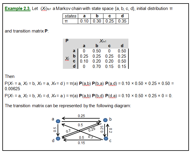
The transition matrix of Example 2.2 can be represented by the following diagram, the transition graph:
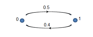
where nodes represent the states of the Markov chain, and arrows represent transition probabilities. The previous graph means that we move from state 0 to state 1 with probability 0.5, and we go back with probability 0.4.
This diagram makes clear that the transition matrix needs not to be symmetrical, that is P(xi, xk) can differ from P(xk, xi).