The output interpretation and test of robustness

Obtaining the final model and Interpretation of the results - Step 3/6

It might be convenient to plot the output in a binary format (presence/absence). The threshold for presence was calculated using the TSS metrics as specified in the BIOMOD_EnsembleForecasting() function (see biomod2 help for details). Being these maps made of zeros and ones, we will not produce a weighted mean, but we will sum them and retain as cells of predicted presence just those where at least 2 of the 3 binary maps predicted the species as present. We first load the binary maps:

> b<-list.files(getwd(), "ensemble_TSSbin.gri", recursive=T, full.names=T)
> b_current<-lapply(grep("current", b, value=T), stack)
> b_future<-lapply(grep("future", b, value=T), stack)

Retain only maps obtained by using TSS as evaluation metrics:

> b_current<-lapply(b_current, "[[", c(2))
> b_future<-lapply(b_future, "[[", c(2))

Finally, we sum the cells that predicted the presence of the species in at least 2 replicates

> b_current<-sum(stack(b_current))
> values(b_current)[values(b_current)%in%c(0:1)]<-0
> values(b_current)[values(b_current)%in%c(2:3)]<-1
> b_future<-sum(stack(b_future))
> values(b_future)[values(b_future)%in%c(0:1)]<-0
> values(b_future)[values(b_future)%in%c(2:3)]<-1

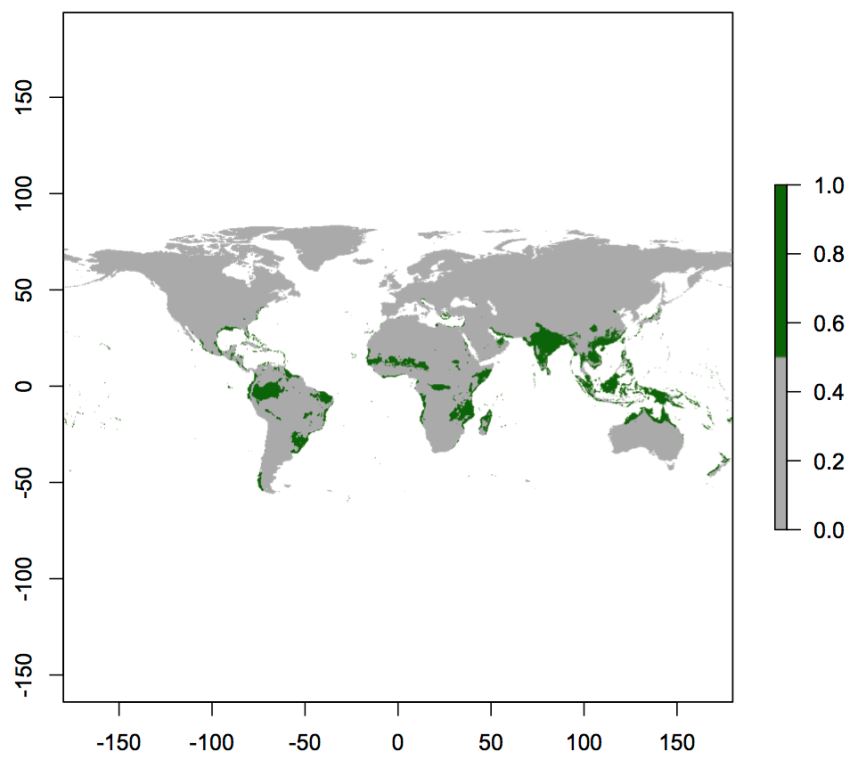
Plot the resulting map of presence/absence under current climate

> plot(b_current, col=c("darkgrey", "darkgreen"))