The output interpretation and test of robustness

Obtaining the final model and Interpretation of the results - Step 2/6

Now we load the six ensembles, 3 for the current and 3 for future climate conditions, and perform the weighted mean with the “TSS” object as weight.

> m<-list.files(getwd(), "ensemble.gri", recursive=T, full.names=T)
> m_current<-lapply(grep("current", m, value=T), stack)
> m_future<-lapply(grep("future", m, value=T), stack)

Here we have 2 esemble models for each replicates. We want only those obtained using TSS as evaluation metrics

> m_current<-lapply(m_current, "[[", c(2))
> m_future<-lapply(m_future, "[[", c(2))

Finally we compute the final ensemble model by averaging the three ensemble models by weighting them according to the respective TSS values

> current_final<-weighted.mean(stack(m_current), w=TSS)
> future_final<-weighted.mean(stack(m_future), w=TSS)

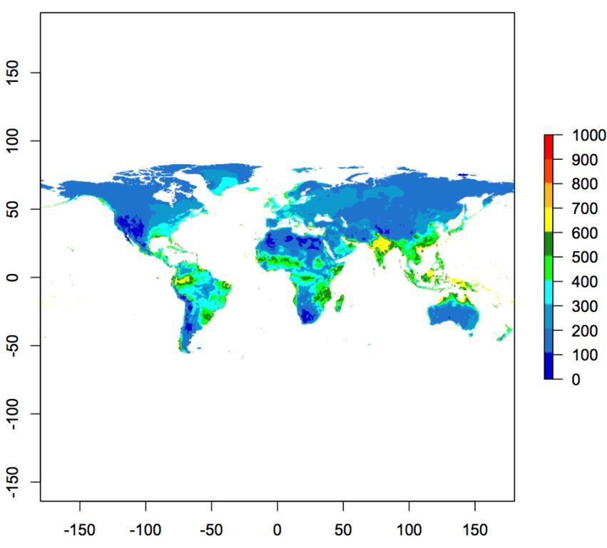
To obtain maps of the final models, we provided in the tutorial a script with a palette function the reproduce the same colour scale used by the MAXENT software. The function requires the minimum and maximum value of the raster intended to be plotted and the interval of values used to shift from a colour to another.

> source("script/palette_MAXENT.R")
> plot(current_final, col=palette_MAXENT(min=0, max=1000, interval=100)[[1]], breaks=palette_MAXENT(0, 1000, 100)[[2]])