The environmental variables

Preparing the model training area

Because P. krameri was not originally distributed worldwide, and we want to create a SDM that take into account the native range of the species, we are going to crop the bioclimatic rasters to create the area used to train the model.

First we will create a buffer around our occurrences points:

>library(rgeos)
>buff<-gBuffer(SpatialPoints(do.call(rbind, krameri)), width=res(r)[1]*100)

The resolution of bioclimatic layers (r) is almost 5 km --> 5km*100=500km

Then, we crop the original layers to the training area delimited by the buffer

>vars<-crop(r, buff, progress="text")
>vars<-mask(vars, buff, progress="text")

Finally we plot the results:

>plot(vars[[1]])
>plot(wrld_simpl, add = T, border = "grey", col = "grey")
>plot(vars[[1]], add=T)

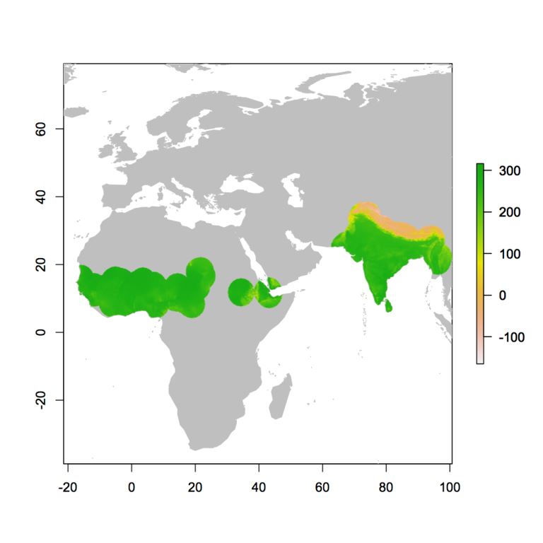
Figure 2.5: Training area

Figure 2.5 shows the bioclimatic variable bio1 (average annual temperature) cropped to the area that we want to use for the training of the model. The same cropping procedure was applied to the other bioclimatic variables.